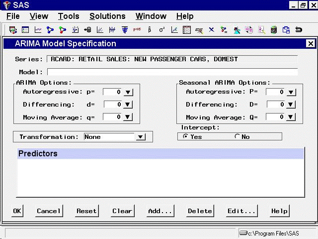
To fit ARIMA or Box-Jenkins models not already provided in the Models to Fit window, select the ARIMA model item from the pop-up menu, toolbar, or Edit menu. This opens the ARIMA Model Specification window, as shown in Figure 47.13.

This ARIMA Model Specification window is structured according to the Box and Jenkins approach to time series modeling. You can specify the same time series models with the Custom Model Specification window and the ARIMA Model Specification window, but the windows are structured differently, and you may find one more convenient than the other.

At the top of the ARIMA Model Specification window is the name and label of the series and the label of the model you are specifying. The model label is filled in with an automatically generated label as you specify options. You can type over the automatic label with your own label for the model. To restore the automatic label, enter a blank label.

Using the ARIMA Model Specification window, you can specify autoregressive (p), differencing (d), and moving average (q) orders for both simple and seasonal factors. You can specify transformations with the Transformation list. You can also specify whether an intercept is included in the ARIMA model.

In addition to specifying seasonal and nonseasonal ARIMA processes, you can also specify predictor variables and other terms as inputs to the model. ARIMA models with inputs are sometimes called ARIMAX models or Box-Tiao models. Another term for this kind of model is dynamic regression.

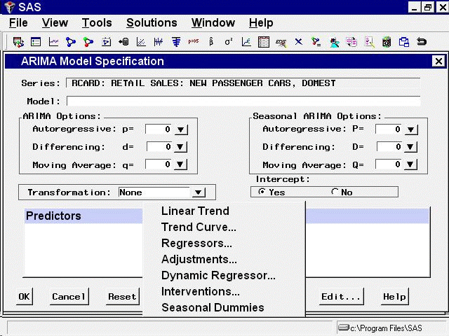
In the lower part of the ARIMA Model Specification window is the list of predictors to the model (initially empty). You can specify predictors by using the Add button. This opens a menu of different kinds of independent effects, as shown in Figure 47.14.

The kinds of predictor effects allowed include time trends, regressors, adjustments, dynamic regression (transfer functions), intervention effects, and seasonal dummy variables. How to use different kinds of predictors is explained in Chapter 49: Using Predictor Variables.

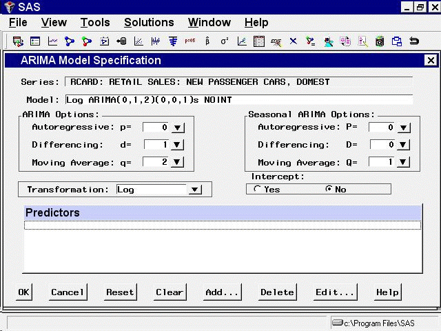
As an example, in the ARIMA Options box, set the order of differencing d to 1 and the moving average order q to 2. You can either type in these values or click the arrows and select the values from pop-up lists.

These selections specify an ARIMA(0,1,2) or IMA(1,2) model. (See Chapter 7: The ARIMA Procedure, for more information about the notation used for ARIMA models.) Notice that the model label at the top is now IMA(1,2) NOINT, meaning that the data are differenced once and a second-order moving-average term is included with no intercept.

In the Seasonal ARIMA Options box, set the seasonal moving-average order Q to 1. This adds a first-order moving-average term at the seasonal (12 month) lag. Finally, select “Log” in the Transformation combo box.

The model label is now Log ARIMA(0,1,2)(0,0,1)s NOINT, and the window appears as shown in Figure 47.15.

Select the OK button to fit the model. The model is fit and added to the Develop Models table.