Creating Paneled Scatter Plots

The SGSCATTER procedure creates a paneled graph for multiple combinations of variables.
The procedure syntax supports the following features:
  • three types of graph layouts: PLOT, COMPARE, and MATRIX
  • basic scatter plots
  • fit and confidence plots: loess curves, regression curves, penalized B-spline curves, and ellipses
  • distribution plots: histograms and density curves (in the diagonal cells of a matrix)
  • legends
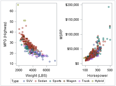
The following example creates a panel using the PLOT layout. The PLOT statement creates a paneled graph of scatter plots where each cell has its own independent set of axes.
SGSCATTER Plot Panel
proc sgscatter data=sashelp.cars;
  plot mpg_highway*weight msrp*horsepower
          / group=type;
run;
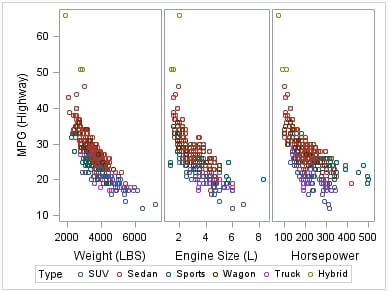
The following example creates a panel using the COMPARE layout. The COMPARE statement creates a paneled graph that uses common axes for each row and column of cells. Cells are created for all crossing of the X and Y variables.
SGSCATTER Compare Panel
proc sgscatter data=sashelp.cars;
  compare y=mpg_highway
          x=(weight enginesize horsepower )
          / group=type;
run;
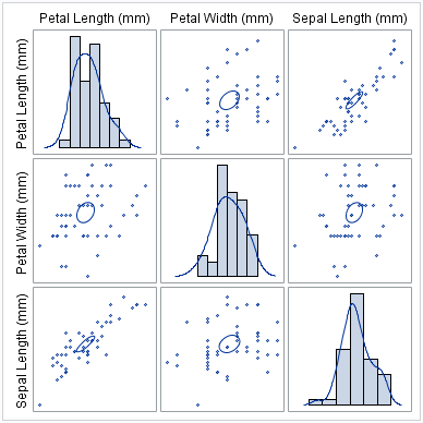
The following example creates a panel using the MATRIX layout. The MATRIX statement creates a matrix of scatter plots where each cell represents a different combination of variables. In the diagonal cells, you can place labels or histograms with or without density curves.
SGSCATTER MATRIX example graph
proc sgscatter data=sashelp.iris
               (where=(species eq "Virginica"));
matrix petallength petalwidth sepallength
       / ellipse=(type=mean)
         diagonal=(histogram kernel);
run;
For more information about the SGSCATTER procedure and the procedure syntax, see SGSCATTER Procedure.