Robust Regression Examples

Diagnostic Plots for Robust Regression

This section is based on Rousseeuw and Van Zomeren (1990). Observations $\mb{x}_ i$ , which are far away from most of the other observations, are called leverage points. One classical method inspects the Mahalanobis distances $MD_ i$ to find outliers $\mb{x}_ i$ ,

$MD_ i = \sqrt {(\mb{x}_ i - \mu ) \mb{C}^{-1}(\mb{x}_ i - \mu )^ T}$

where $\mb{C}$ is the classical sample covariance matrix.

Note that the MVE and MCD subroutines compute the classical Mahalanobis distances $MD_ i$ together with the robust distances $RD_ i$ . In classical linear regression, the diagonal elements $h_{ii}$ of the hat matrix,

$\mb{H} = \mb{X}(\mb{X}^ T\mb{X})^{-1}\mb{X}^ T$

are used to identify leverage points. Rousseeuw and Van Zomeren (1990) report the following monotone relationship between the $h_{ii}$ and $MD_ i$ :

$h_{ii} = \frac{(MD_ i)^2}{N-1} + \frac{1}{n}$

They point out that neither the $MD_ i$ nor the $h_{ii}$ are entirely safe for detecting leverage points reliably. Multiple outliers do not necessarily have large $MD_ i$ values because of the masking effect.

Therefore, the definition of a leverage point is based entirely on the outlyingness of $\mb{x}_ i$ and is not related to the response value $y_ i$ . By including the $y_ i$ value in the definition, Rousseeuw and Van Zomeren (1990) distinguish between the following:

Good leverage points are points $(\mb{x}_ i,y_ i)$ that are close to the regression plane; that is, good leverage points improve the precision of the regression coefficients.
Bad leverage points are points $(\mb{x}_ i,y_ i)$ that are far from the regression plane; that is, bad leverage points reduce the precision of the regression coefficients.

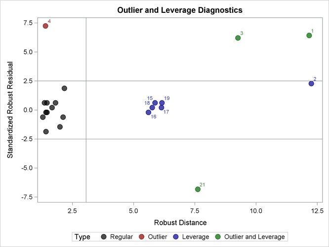
Rousseeuw and Van Zomeren (1990) propose plotting the standardized residuals of robust regression (LMS or LTS) versus the robust distances that are obtained from MVE or MCD. Two horizontal lines that correspond to residual values of $+2.5$ and $-2.5$ are useful for distinguishing between small and large residuals, and one vertical line that corresponds to the $\sqrt {\chi ^2_{n,.975}}$ is used to distinguish between small and large distances.

For example, once again consider the stack loss data from Brownlee (1965). The following statements call the RDPLOT module, which is distributed in the RobustMC.sas file. As in the previous section, the LOAD MODULES=_ALL_ statement loads modules that are defined in the RobustMC.sas file.

%include "C:\<path>\RobustMC.sas";
proc iml;
load module=_all_;

   /* Obs X1  X2  X3   Y  Stack Loss data */
SL = { 1  80  27  89  42,
       2  80  27  88  37,
       3  75  25  90  37,
       4  62  24  87  28,
       5  62  22  87  18,
       6  62  23  87  18,
       7  62  24  93  19,
       8  62  24  93  20,
       9  58  23  87  15,
      10  58  18  80  14,
      11  58  18  89  14,
      12  58  17  88  13,
      13  58  18  82  11,
      14  58  19  93  12,
      15  50  18  89   8,
      16  50  18  86   7,
      17  50  19  72   8,
      18  50  19  79   8,
      19  50  20  80   9,
      20  56  20  82  15,
      21  70  20  91  15 };
x = SL[, 2:4]; y = SL[, 5];

LMSOpt = j(9,1,.);
MCDOpt = j(5,1,.);
MCDOpt[5]= -1;             /* nrep: all subsets */

run RDPlot("LMS", LMSOpt, MCDOpt, y, x);

The diagnostic plot is shown in Output 12.27. The graph shows the standardized LMS residuals plotted against the robust distances $RD_ i$ . The plot shows that observation 4 is a regression outlier but not a leverage point, so it is a vertical outlier. Observations 1, 3, and 21 are bad leverage points, whereas observation 2 is a good leverage point. Notice that observation 2 is very close to the boundary between good and bad leverage points.

Output 12.27: Stack Loss Data: LMS Residuals versus Robust Distances

If you use the LTS algorithm instead of the LMS algorithm, observation 13 is classified as a vertical outlier and observation 2 is classified as a bad leverage point.