The SHEWHART Procedure

Diagnosing and Modeling Autocorrelation

You can diagnose autocorrelation with an autocorrelation plot created with the ARIMA procedure.

ods graphics on;
ods select ChiSqAuto SeriesACFPlot SeriesPACFPlot;
proc arima data=Chemical plots(only)=series(acf pacf);
   identify var = xt;
run;
quit;

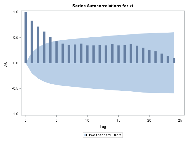
Refer to SAS/ETS User's Guide for details on the ARIMA procedure. The output, shown in Figure 17.192 and Figure 17.193, indicates that the data are highly autocorrelated with a lag 1 autocorrelation of 0.83.

Figure 17.192: Autocorrelation Check for Chemical Data

Individual Measurements Chart

The ARIMA Procedure

Autocorrelation Check for White Noise
To Lag	Chi-Square	DF	Pr > ChiSq	Autocorrelations
6	228.15	6	<.0001	0.830	0.718	0.619	0.512	0.426	0.381
12	315.34	12	<.0001	0.360	0.364	0.380	0.347	0.348	0.354
18	406.76	18	<.0001	0.349	0.371	0.348	0.353	0.368	0.341
24	442.15	24	<.0001	0.303	0.261	0.230	0.184	0.141	0.098

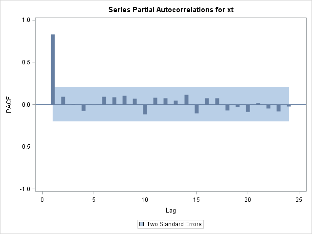
Figure 17.193: Autocorrelation Plots for Chemical Data

The partial autocorrelation plot in Figure 17.193 suggests that the data can be modeled with a first-order autoregressive model, commonly referred to as an AR(1) model.

$\tilde{x}_{t} \equiv x_{t} - \mu = \phi _{0} + \phi _{1} \tilde{x}_{t-1} + \epsilon _{t}$

You can fit this model with the ARIMA procedure. The results in Figure 17.194 show that the equation of the fitted model is $\tilde{x}_{t} = 13.05 + 0.847 \tilde{x}_{t-1}$ .

ods select ParameterEstimates;
proc arima data=Chemical;
   identify var=xt;
   estimate p=1 method=ml;
run;

Figure 17.194: Fitted AR(1) Model

Individual Measurements Chart

The ARIMA Procedure

Maximum Likelihood Estimation
Parameter	Estimate	Standard Error	t Value	Approx Pr > \|t\|	Lag
MU	85.28375	2.32973	36.61	<.0001	0
AR1,1	0.84694	0.05221	16.22	<.0001	1