The GLMSELECT Procedure

Elastic Net Selection (ELASTICNET)

The elastic net method bridges the LASSO method and ridge regression. It balances having a parsimonious model with borrowing strength from correlated regressors, by solving the least squares regression problem with constraints on both the sum of the absolute coefficients and the sum of the squared coefficients. More specifically, the elastic net coefficients $\bbeta = (\beta _1,\beta _2,\ldots ,\beta _ m)$ are the solution to the constrained optimization problem

$\mbox{minimize} ||\mb {y}-\bX \bbeta ||^2 \qquad \mbox{subject to} \quad \sum _{j=1}^{m} |\beta _ j | \leq t_1, \sum _{j=1}^{m} \beta _ j^2 \leq t_2$

The method can be written as the equivalent Lagrangian form

$\mbox{minimize} ||\mb {y}-\bX \bbeta ||^2 + \lambda _1 \sum _{j=1}^{m} |\beta _ j | + \lambda _2 \sum _{j=1}^{m} \beta _ j^2$

If $t_1$ is set to a very large value or, equivalently, if $\lambda _1$ is set to 0, then the elastic net method reduces to ridge regression. If $t_2$ is set to a very large value or, equivalently, if $\lambda _2$ is set to 0, then the elastic net method reduces to LASSO. If $t_1$ and $t_2$ are both large or, equivalently, if $\lambda _1$ and $\lambda _2$ are both set to 0, then the elastic net method reduces to ordinary least squares regression.

As stated by Zou and Hastie (2005), the elastic net method can overcome the limitations of LASSO in the following three scenarios:

In the case where you have more parameters than observations, $m >n$ , the LASSO method selects at most $n$ variables before it saturates, because of the nature of the convex optimization problem. This can be a defect for a variable selection method. By contrast, the elastic net method can select more than $n$ variables in this case because of the ridge regression regularization.
If there is a group of variables that have high pairwise correlations, then whereas LASSO tends to select only one variable from that group, the elastic net method can select more than one variable.
In the $n >m$ case, if there are high correlations between predictors, it has been empirically observed that the prediction performance of LASSO is dominated by ridge regression. In this case, the elastic net method can achieve better prediction performance by using ridge regression regularization.

An elastic net fit is achieved by building on LASSO estimation, in the following sense. Let $\tilde{ \bX }$ be a matrix obtained by augmenting $\bX$ with a scaled identity matrix,

$\tilde{ \bX } =[\bX ; \sqrt {\lambda _2} I]$

Let $\tilde{\mb { y}}$ be a vector correspondingly obtained by augmenting the response $\mb {y}$ with $m$ 0’s,

$\tilde{\mb {y}} =[\mb {y}; \mb {0}]$

Then the Lagrangian form of the elastic net optimization problem can be reformulated as

$\mbox{minimize} ||\tilde{\mb {y}}- \tilde{\bX } \bbeta ||^2 + \lambda _1 \sum _{j=1}^{m} |\beta _ j |$

In other words, you can solve the elastic net method in the same way as LASSO by using this augmented design matrix $\tilde{\bX }$ and response $\tilde{\mb {y}}$ . Therefore, for given $\lambda _2$ , the coefficients of the elastic net fit follow the same piecewise linear path as LASSO. Zou and Hastie (2005) suggest rescaling the coefficients by $1+\lambda _2$ to deal with the double amount of shrinkage in the elastic net fit, and such rescaling is applied when you specify the ENSCALE option in the MODEL statement.

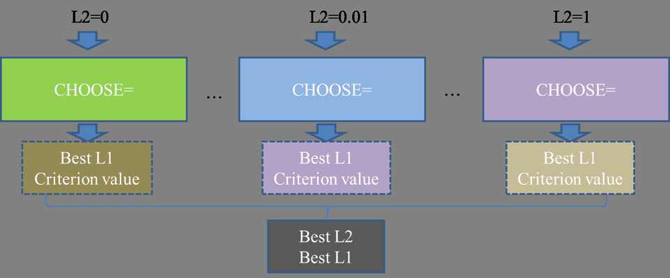
If you have a good estimate of $\lambda _2$ , you can specify the value in the L2= option. If you do not specify a value for $\lambda _2$ , then by default PROC GLMSELECT searches for a value between 0 and 1 that is optimal according to the current CHOOSE= criterion. Figure 47.12 illustrates the estimation of the ridge regression parameter $\lambda _2$ (L2). Meanwhile, if you do not specify the CHOOSE= option, then the model at the final step in the selection process is selected for each $\lambda _2$ (L2), and the criterion value shown in Figure 47.12 is the one at the final step that corresponds to the specified STOP= option (STOP=SBC by default).

Figure 47.12: Estimation of the Ridge Regression Parameter $\lambda _2$ (L2) in the Elastic Net Method

Note that when you specify the L2SEARCH=GOLDEN, it is assumed that the criterion curve that corresponds to the CHOOSE= option with respect to $\lambda _2$ is a smooth and bowl-shaped curve. However, this assumption is not checked and validated. Hence, the default value for the L2SEARCH= option is set to GRID.