Finding the Least Squares Estimators :: SAS/STAT(R) 13.1 User's Guide

Finding the Least Squares Estimators

Finding the least squares estimator of $\bbeta$ can be motivated as a calculus problem or by considering the geometry of least squares. The former approach simply states that the OLS estimator is the vector $\widehat{\bbeta }$ that minimizes the objective function

$\mr {SSE} = \left(\bY -\bX \bbeta \right)’\left(\bY -\bX \bbeta \right)$

Applying the differentiation rules from the section Matrix Differentiation leads to

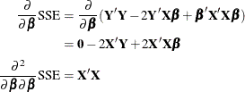
$\begin{align*} \frac{\partial }{\partial \bbeta } \mr {SSE} =& \, \, \frac{\partial }{\partial \bbeta } ( \bY ’\bY - 2\bY ’\bX \bbeta + \bbeta ’\bX ’\bX \bbeta ) \\ =& \, \, \mb {0} - 2\bX ’\bY + 2\bX ’\bX \bbeta \\ \frac{\partial ^2}{\partial \bbeta \partial \bbeta } \mr {SSE} =& \, \, \bX ’\bX \end{align*}$

Consequently, the solution to the normal equations, $\bX ’\bX \bbeta = \bX ’\bY$ , solves $\frac{\partial }{\partial \bbeta } \mr {SSE} = 0$ , and the fact that the second derivative is nonnegative definite guarantees that this solution minimizes $\mr {SSE}$ . The geometric argument to motivate ordinary least squares estimation is as follows. Assume that $\bX$ is of rank k. For any value of $\bbeta$ , such as $\tilde{\bbeta }$ , the following identity holds:

$\bY = \bX \tilde{\bbeta } + \left(\bY -\bX \tilde{\bbeta }\right)$

The vector $\bX \tilde{\bbeta }$ is a point in a k-dimensional subspace of $R^ n$ , and the residual $(\bY -\bX \tilde{\bbeta })$ is a point in an $(n-k)$ -dimensional subspace. The OLS estimator is the value $\widehat{\bbeta }$ that minimizes the distance of $\bX \tilde{\bbeta }$ from $\bY$ , implying that $\bX \widehat{\bbeta }$ and $(\bY -\bX \widehat{\bbeta })$ are orthogonal to each other; that is,

$(\bY -\bX \widehat{\bbeta })’\bX \widehat{\bbeta } = \mb {0}$ . This in turn implies that $\widehat{\bbeta }$ satisfies the normal equations, since

$\widehat{\bbeta }’\bX ’\bY = \widehat{\bbeta }’\bX ’\bX \widehat{\bbeta } \Leftrightarrow \bX ’\bX \widehat{\bbeta } = \bX ’\bY$

Full-Rank Case

If $\bX$ is of full column rank, the OLS estimator is unique and given by

$\widehat{\bbeta } = \left(\bX ’\bX \right)^{-1}\bX ’\bY$

The OLS estimator is an unbiased estimator of $\bbeta$ —that is,

$\begin{align*} \mr {E}[\widehat{\bbeta }] =& \mr {E}\left[\left(\bX ’\bX \right)^{-1}\bX ’\bY \right] \\ =& \left(\bX ’\bX \right)^{-1}\bX ’\mr {E}[\bY ] = \left(\bX ’\bX \right)^{-1}\bX ’\bX \bbeta = \bbeta \end{align*}$

Note that this result holds if $\mr {E}[\bY ] = \bX \bbeta$ ; in other words, the condition that the model errors have mean zero is sufficient for the OLS estimator to be unbiased. If the errors are homoscedastic and uncorrelated, the OLS estimator is indeed the best linear unbiased estimator (BLUE) of $\bbeta$ —that is, no other estimator that is a linear function of $\bY$ has a smaller mean squared error. The fact that the estimator is unbiased implies that no other linear estimator has a smaller variance. If, furthermore, the model errors are normally distributed, then the OLS estimator has minimum variance among all unbiased estimators of $\bbeta$ , whether they are linear or not. Such an estimator is called a uniformly minimum variance unbiased estimator, or UMVUE.

Rank-Deficient Case

In the case of a rank-deficient $\bX$ matrix, a generalized inverse is used to solve the normal equations:

$\widehat{\bbeta } = \left(\bX ’\bX \right)^{-}\bX ’\bY$

Although a $g_1$ -inverse is sufficient to solve a linear system, computational expedience and interpretation of the results often dictate the use of a generalized inverse with reflexive properties (that is, a $g_2$ -inverse; see the section Generalized Inverse Matrices for details). Suppose, for example, that the $\bX$ matrix is partitioned as $\bX = \left[\bX _1 \, \, \bX _2\right]$ , where $\bX _1$ is of full column rank and each column in $\bX _2$ is a linear combination of the columns of $\bX _1$ . The matrix

$\mb {G}_1 = \left[\begin{array}{cc} \left(\bX _1’\bX _1\right)^{-1} & \left(\bX _1’\bX _1\right)^{-1}\bX _1’\bX _2 \cr -\bX _2’\bX _1\left(\bX _1’\bX _1\right)^{-1} & \mb {0} \end{array}\right]$

is a $g_1$ -inverse of $\bX ’\bX$ and

$\mb {G}_2 = \left[\begin{array}{cc} \left(\bX _1’\bX _1\right)^{-1} & \mb {0} \cr \mb {0} & \mb {0} \end{array}\right]$

is a $g_2$ -inverse. If the least squares solution is computed with the $g_1$ -inverse, then computing the variance of the estimator requires additional matrix operations and storage. On the other hand, the variance of the solution that uses a $g_2$ -inverse is proportional to $G_2$ .

$\begin{align*} \mr {Var}\left[\bG _1\bX ’\bY \right] =& \, \, \sigma ^2 \bG _1\bX ’\bX \mb {G}_1 \\ \mr {Var}\left[\bG _2\bX ’\bY \right] =& \, \, \sigma ^2 \bG _2\bX ’\bX \bG _2 = \sigma ^2\bG _2 \end{align*}$

If a generalized inverse $\bG$ of $\bX ’\bX$ is used to solve the normal equations, then the resulting solution is a biased estimator of $\bbeta$ (unless $\bX ’\bX$ is of full rank, in which case the generalized inverse is “the” inverse), since $\mr {E}\left[\widehat{\bbeta }\right] = \bG \bX ’\bX \bbeta$ , which is not in general equal to $\bbeta$ .

If you think of estimation as “estimation without bias,” then $\widehat{\bbeta }$ is the estimator of something, namely $\bG \bX \bbeta$ . Since this is not a quantity of interest and since it is not unique—it depends on your choice of $\bG$ —Searle (1971, p. 169) cautions that in the less-than-full-rank case, $\widehat{\bbeta }$ is a solution to the normal equations and “nothing more.”