Introduction to Structural Equation Modeling with Latent Variables

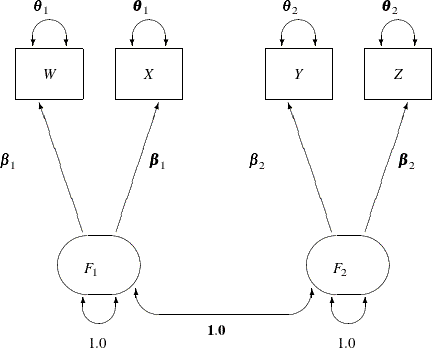
H1: One-Factor Model with Parallel Tests for Lord Data

The path diagram for the one-factor model with parallel tests is shown in Figure 17.29.

Figure 17.29: H1: One-Factor Model with Parallel Tests for Lord Data

The hypothesis $H_{1}$ differs from $H_{2}$ in that F1 and F2 have a perfect correlation in $H_{1}$ . This is indicated by the fixed value 1.0 for the double-headed path that connects F1 and F2 in Figure 17.29. Again, you need only minimal modification of the preceding specification for $H_{2}$ to specify the path diagram in Figure 17.29, as shown in the following statements:

proc calis data=lord;
   path
      W <=== F1   = beta1,
      X <=== F1   = beta1,
      Y <=== F2   = beta2,
      Z <=== F2   = beta2;
   pvar
      F1  = 1.0,
      F2  = 1.0,
      W X = 2 * theta1,
      Y Z = 2 * theta2;
   pcov
      F1 F2 = 1.0;
run;

The only modification of the preceding specification is in the PCOV statement, where you put a constant 1 for the covariance between F1 and F2. An annotated fit summary is displayed in Figure 17.30.

Figure 17.30: Fit Summary, H1: One-Factor Model with Parallel Tests for Lord Data

Fit Summary
Chi-Square	37.3337
Chi-Square DF	6
Pr > Chi-Square	<.0001
Standardized RMR (SRMR)	0.0286
Adjusted GFI (AGFI)	0.9509
RMSEA Estimate	0.0898
Bentler Comparative Fit Index	0.9785

The chi-square value is 37.3337 (df=6, p<0.0001). This indicates that you can reject the hypothesized model H1 at the 0.01 $\alpha$ -level. The standardized root mean square error (SRMSR) is 0.0286, the adjusted GFI (AGFI) is 0.9509, and Bentler’s comparative fit index is 0.9785. All these indicate good model fit. However, the RMSEA is 0.0898, which does not support an acceptable model for the data.

The estimation results are displayed in Figure 17.31.

Figure 17.31: Estimation Results, H1: One-Factor Model with Parallel Tests for Lord Data

PATH List
Path			Parameter	Estimate	Standard Error	t Value	Pr > \|t\|
W	<===	F1	beta1	7.18623	0.26598	27.0180	<.0001
X	<===	F1	beta1	7.18623	0.26598	27.0180	<.0001
Y	<===	F2	beta2	8.44198	0.28000	30.1494	<.0001
Z	<===	F2	beta2	8.44198	0.28000	30.1494	<.0001

Variance Parameters
Variance Type	Variable	Parameter	Estimate	Standard Error	t Value	Pr > \|t\|
Exogenous	F1		1.00000
	F2		1.00000
Error	W	theta1	34.68865	1.64634	21.0701	<.0001
	X	theta1	34.68865	1.64634	21.0701	<.0001
	Y	theta2	26.28513	1.39955	18.7812	<.0001
	Z	theta2	26.28513	1.39955	18.7812	<.0001

Covariances Among Exogenous Variables
Var1	Var2	Estimate	Standard Error	t Value	Pr > \|t\|
F1	F2	1.00000

The goodness-of-fit tests for the four hypotheses are summarized in the following table.

	Number of		Degrees of
Hypothesis	Parameters	$\chi ^2$	Freedom	p-value	$\hat{\rho }$
$H_{1}$	4	37.33	6	< .0001	1.0
$H_{2}$	5	1.93	5	0.8583	0.8986
$H_{3}$	8	36.21	2	< .0001	1.0
$H_{4}$	9	0.70	1	0.4018	0.8986

Recall that the estimates of $\rho$ for $H_{2}$ and $H_{4}$ are almost identical, about 0.90, indicating that the speeded and unspeeded tests are measuring almost the same latent variable. However, when $\rho$ was set to 1 in $H_{1}$ and $H_{3}$ (both one-factor models), both hypotheses were rejected. Hypotheses $H_{2}$ and $H_{4}$ (both two-factor models) seem to be consistent with the data. Since $H_{2}$ is obtained by adding four constraints (for the requirement of parallel tests) to $H_{4}$ (the full model), you can test $H_{2}$ versus $H_{4}$ by computing the differences of the chi-square statistics and their degrees of freedom, yielding a chi-square of 1.23 with four degrees of freedom, which is obviously not significant. In a sense, the chi-square difference test means that representing the data by $H_{2}$ would not be significantly worse than representing the data by $H_{4}$ . In addition, because $H_{2}$ offers a more precise description of the data (with the assumption of parallel tests) than $H_{4}$ , it should be chosen because of its simplicity. In conclusion, the two-factor model with parallel tests provides the best explanation of the data.