The SEVERITY Procedure
- Overview
-
Getting Started

-
Syntax
-
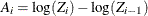
DetailsPredefined DistributionsCensoring and TruncationParameter Estimation MethodParameter InitializationEstimating Regression EffectsEmpirical Distribution Function Estimation MethodsStatistics of FitDefining a Distribution Model with the FCMP ProcedurePredefined Utility FunctionsCustom Objective FunctionsMultithreaded ComputationInput Data SetsOutput Data SetsDisplayed OutputODS Graphics
-
Examples
- References
Statistics of Fit
PROC SEVERITY computes and reports various statistics of fit to indicate how well the estimated model fits the data. The statistics belong to two categories: likelihood-based statistics and EDF-based statistics. Statistics Neg2LogLike, AIC, AICC, and BIC are likelihood-based statistics, and statistics KS, AD, and CvM are EDF-based statistics. The following subsections provide definitions of each.
Likelihood-Based Statistics
Let ![]() denote the response variable values. Let
denote the response variable values. Let ![]() be the likelihood as defined in the section Likelihood Function. Let
be the likelihood as defined in the section Likelihood Function. Let ![]() denote the number of model parameters estimated. Note that
denote the number of model parameters estimated. Note that ![]() , where
, where ![]() is the number of distribution parameters,
is the number of distribution parameters, ![]() is the number of regressors, if any, specified in the SCALEMODEL statement, and
is the number of regressors, if any, specified in the SCALEMODEL statement, and ![]() is the number of regressors found to be linearly dependent (redundant) on other regressors. Given this notation, the likelihood-based
statistics are defined as follows:
is the number of regressors found to be linearly dependent (redundant) on other regressors. Given this notation, the likelihood-based
statistics are defined as follows:
- Neg2LogLike
-
The log likelihood is reported as
![\[ \text {Neg2LogLike} = -2 \log (L) \]](images/etsug_severity0533.png)
The multiplying factor
 makes it easy to compare it to the other likelihood-based statistics. A model with a smaller value of Neg2LogLike is deemed
better.
makes it easy to compare it to the other likelihood-based statistics. A model with a smaller value of Neg2LogLike is deemed
better.
- AIC
-
The Akaike’s information criterion (AIC) is defined as
![\[ \text {AIC} = -2 \log (L) + 2 p \]](images/etsug_severity0535.png)
A model with a smaller value of AIC is deemed better.
- AICC
-
The corrected Akaike’s information criterion (AICC) is defined as
![\[ \text {AICC} = -2 \log (L) + \frac{2 N p}{N - p - 1} \]](images/etsug_severity0536.png)
A model with a smaller value of AICC is deemed better. It corrects the finite-sample bias that AIC has when
 is small compared to
  . AICC is related to AIC as
![\[ \text {AICC} = \text {AIC} + \frac{2p(p+1)}{N-p-1} \]](images/etsug_severity0537.png)
As
becomes large compared to , AICC converges to AIC. AICC is usually recommended over AIC as a model selection criterion.
- BIC
-
The Schwarz Bayesian information criterion (BIC) is defined as
![\[ \text {BIC} = -2 \log (L) + p \log (N) \]](images/etsug_severity0538.png)
A model with a smaller value of BIC is deemed better.
EDF-Based Statistics
This class of statistics is based on the difference between the estimate of the cumulative distribution function (CDF) and
the estimate of the empirical distribution function (EDF). Let ![]() denote the sample of
denote the sample of ![]() values of the response variable. Let
values of the response variable. Let ![]() denote the number of observations with a value less than or equal to
denote the number of observations with a value less than or equal to ![]() , where
, where ![]() is an indicator function. Let
is an indicator function. Let ![]() denote the EDF estimate that is computed by using the method specified in the EMPIRICALCDF= option. Let
denote the EDF estimate that is computed by using the method specified in the EMPIRICALCDF= option. Let ![]() denote the estimate of the CDF. Let
denote the estimate of the CDF. Let ![]() denote the EDF estimate of
denote the EDF estimate of ![]() values that are computed using the same method that is used to compute the EDF of
values that are computed using the same method that is used to compute the EDF of ![]() values. Using the probability integral transformation, if
values. Using the probability integral transformation, if ![]() is the true distribution of the random variable
is the true distribution of the random variable ![]() , then the random variable
, then the random variable ![]() is uniformly distributed between 0 and 1 (D’Agostino and Stephens 1986, Ch. 4). Thus, comparing
is uniformly distributed between 0 and 1 (D’Agostino and Stephens 1986, Ch. 4). Thus, comparing ![]() with
with ![]() is equivalent to comparing
is equivalent to comparing ![]() with
with ![]() (uniform distribution).
(uniform distribution).
Note the following two points regarding which CDF estimates are used for computing the test statistics:
-
If regressor variables are specified, then the CDF estimates
 used for computing the EDF test statistics are from a mixture distribution. See the section CDF and PDF Estimates with Regression Effects for more information.
-
If the EDF estimates are conditional because of the truncation information, then each unconditional estimate
is converted to a conditional estimate using the method described in the section Truncation and Conditional CDF Estimates.
In the following, it is assumed that ![]() denotes an appropriate estimate of the CDF if truncation or regression effects are specified. Given this, the EDF-based statistics
of fit are defined as follows:
denotes an appropriate estimate of the CDF if truncation or regression effects are specified. Given this, the EDF-based statistics
of fit are defined as follows:
- KS
-
The Kolmogorov-Smirnov (KS) statistic computes the largest vertical distance between the CDF and the EDF. It is formally defined as follows:
![\[ \text {KS} = \sup _ y | F_ n(y) - F(y) | \]](images/etsug_severity0549.png)
If the STANDARD method is used to compute the EDF, then the following formula is used:


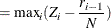

Note that
 is assumed to be 0.
If the method used to compute the EDF is any method other than the STANDARD method, then the following formula is used:


- AD
-
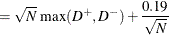
The Anderson-Darling (AD) statistic is a quadratic EDF statistic that is proportional to the expected value of the weighted squared difference between the EDF and CDF. It is formally defined as follows:
![\[ \text {AD} = N \int _{-\infty }^{\infty } \frac{(F_ n(y) - F(y))^2}{F(y) (1-F(y))} dF(y) \]](images/etsug_severity0561.png)
If the STANDARD method is used to compute the EDF, then the following formula is used:
![\[ \text {AD} = -N - \frac{1}{N} \sum _{i=1}^{N} \left[ (2 r_ i - 1) \log (Z_ i) + (2 N + 1 - 2 r_ i) \log (1-Z_ i) \right] \]](images/etsug_severity0562.png)
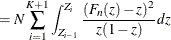
If the method used to compute the EDF is any method other than the STANDARD method, then the statistic can be computed by using the following two pieces of information:
-
If the EDF estimates are computed using the KAPLANMEIER or MODIFIEDKM methods, then EDF is a step function such that the estimate
 is a constant equal to
  in interval
 ![$[Z_{i-1}, Z_ i]$](images/etsug_severity0565.png) . If the EDF estimates are computed using the TURNBULL method, then there are two types of intervals: one in which the EDF
curve is constant and the other in which the EDF curve is theoretically undefined. For computational purposes, it is assumed
that the EDF curve is linear for the latter type of the interval. For each method, the EDF estimate
. If the EDF estimates are computed using the TURNBULL method, then there are two types of intervals: one in which the EDF
curve is constant and the other in which the EDF curve is theoretically undefined. For computational purposes, it is assumed
that the EDF curve is linear for the latter type of the interval. For each method, the EDF estimate  at
at  can be written as
![\[ F_ n(z) = F_ n(Z_{i-1}) + S_ i (z - Z_{i-1}), \text { for } z \in [Z_{i-1},Z_ i] \]](images/etsug_severity0566.png)
where
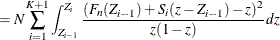
 is the slope of the line defined as
![\[ S_ i = \frac{F_ n(Z_{i})-F_ n(Z_{i-1})}{Z_{i}-Z_{i-1}} \]](images/etsug_severity0568.png)
For the KAPLANMEIER or MODIFIEDKM method,
 in each interval.
-
Using the probability integral transform
 , the formula simplifies to
![\[ \text {AD} = N \int _{-\infty }^{\infty } \frac{(F_ n(z) - z)^2}{z (1-z)} dz \]](images/etsug_severity0571.png)
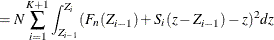
The computation formula can then be derived from the following approximation:


where
 ,
,  , and
, and  is the number of points at which the EDF estimate are computed. For the TURNBULL method,
  for some
  .
.
Assuming
 ,
,  ,
,  , and
, and  yields the following computation formula:
![\begin{equation*} \begin{split} \text {AD} = & - N (Z_1 + \log (1-Z_1) + \log (Z_ K) + (1-Z_ K)) \\ & + N \sum _{i=2}^{K} \left[ P_ i^2 A_ i - (Q_ i-P_ i)^2 B_ i - Q_ i^2 C_ i \right] \end{split}\end{equation*}](images/etsug_severity0584.png)
where
 ,
,  , and
, and  .
.
If EDF estimates are computed using the KAPLANMEIER or MODIFIEDKM method, then
 and
and  , which simplifies the formula as
![\begin{equation*} \begin{split} \text {AD} = & - N (1 + \log (1-Z_1) + \log (Z_ K)) \\ & + N \sum _{i=2}^{K} \left[ F_ n(Z_{i-1})^2 A_ i - (1-F_ n(Z_{i-1}))^2 B_ i \right] \end{split}\end{equation*}](images/etsug_severity0590.png)
-
- CvM
-
The Cramér-von Mises (CvM) statistic is a quadratic EDF statistic that is proportional to the expected value of the squared difference between the EDF and CDF. It is formally defined as follows:
![\[ \text {CvM} = N \int _{-\infty }^{\infty } (F_ n(y) - F(y))^2 dF(y) \]](images/etsug_severity0591.png)
If the STANDARD method is used to compute the EDF, then the following formula is used:
![\[ \text {CvM} = \frac{1}{12 N} + \sum _{i=1}^{N} \left( Z_ i - \frac{(2 r_ i - 1)}{2N}\right)^2 \]](images/etsug_severity0592.png)
If the method used to compute the EDF is any method other than the STANDARD method, then the statistic can be computed by using the following two pieces of information:
-
As described previously for the AD statistic, the EDF estimates are assumed to be piecewise linear such that the estimate
at is
where
is the slope of the line defined as
For the KAPLANMEIER or MODIFIEDKM method,
in each interval.
-
Using the probability integral transform
, the formula simplifies to:
![\[ \text {CvM} = N \int _{-\infty }^{\infty } (F_ n(z) - z)^2 dz \]](images/etsug_severity0593.png)
The computation formula can then be derived from the following approximation:

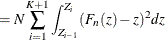
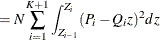
where
, , and is the number of points at which the EDF estimate are computed. For the TURNBULL method, for some .
Assuming
, , and yields the following computation formula:
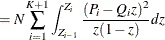
![\[ \text {CvM} = N \frac{Z_1^3}{3} + N \sum _{i=2}^{K+1} \left[ P_ i^2 A_ i - P_ i Q_ i B_ i - \frac{Q_ i^2}{3} C_ i \right] \]](images/etsug_severity0599.png)
where
 ,
,  , and
, and  .
.
If EDF estimates are computed using the KAPLANMEIER or MODIFIEDKM method, then
and , which simplifies the formula as
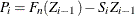
![\[ \text {CvM} = \frac{N}{3} + N \sum _{i=2}^{K+1} \left[ F_ n(Z_{i-1})^2 (Z_ i-Z_{i-1}) - F_ n(Z_{i-1}) (Z_ i^2-Z_{i-1}^2) \right] \]](images/etsug_severity0603.png)
which is similar to the formula proposed by Koziol and Green (1976).
-