The SSM Procedure (Experimental)
-
Overview

- Getting Started
-
Syntax
-
DetailsState Space Model and NotationTypes of Data OrganizationOverview of Model Specification SyntaxLikelihood, Filtering, and SmoothingContrasting PROC SSM with Other SAS Procedures Predefined Trend ModelsPredefined Structural ModelsCovariance ParameterizationMissing ValuesComputational IssuesDisplayed OutputODS Table NamesODS Graph NamesOUT= Data Set
-
ExamplesBivariate Basic Structural Model Two-Way Random-Effects and Autoregressive Model for Panel DataBackcasting, Forecasting, and InterpolationSmoothing of Repeated Measures DataA User-Defined Trend ModelModel with Multiple ARIMA ComponentsDynamic Factor ModelingDiagnostic PlotsVariable Bandwidth Smoothing
- References
Predefined Trend Models
The statistical models that govern the predefined trend components available in the SSM procedure are divided into two groups:
models that are applicable to equally spaced data (possibly with replication), and models that are applicable more generally
(the irregular data type). Each trend component can be described as a dot product ![]() for some (time-invariant) vector
for some (time-invariant) vector ![]() and a state vector
and a state vector ![]() . The component specification is complete after the vector
. The component specification is complete after the vector ![]() is specified and the system matrices that govern the equations of
is specified and the system matrices that govern the equations of ![]() are specified. For trend models for regular data, all the system matrices are time-invariant. For irregular data,
are specified. For trend models for regular data, all the system matrices are time-invariant. For irregular data, ![]() and
and ![]() depend on the spacing between the distinct time points:
depend on the spacing between the distinct time points: ![]() .
.
Trend Models for Regular Data
These models are applicable when the data type is either regular or regular-with-replication. A good reference for these models is Harvey (1989).
Random Walk Trend
This model provides a trend pattern in which the level of the curve changes slowly. The rapidity of this change is inversely
proportional to the disturbance variance ![]() that governs the underlying state. It can be described as
that governs the underlying state. It can be described as ![]() , where
, where ![]() and the (one-dimensional) state
and the (one-dimensional) state ![]() follows a random walk:
follows a random walk:
|
|
Here ![]() and
and ![]() . The initial condition is fully diffuse. Note that if
. The initial condition is fully diffuse. Note that if ![]() , the resulting trend is a fixed constant.
, the resulting trend is a fixed constant.
Local Linear Trend
This model provides a trend pattern in which both the level and the slope of the curve vary slowly. This variation in the
level and the slope is controlled by two parameters: ![]() controls the level variation, and
controls the level variation, and ![]() controls the slope variation. If
controls the slope variation. If ![]() , the resulting trend is called an integrated random walk. If both
, the resulting trend is called an integrated random walk. If both ![]() and
and ![]() , then the resulting model is the deterministic linear time trend. Here
, then the resulting model is the deterministic linear time trend. Here ![]() ,
, ![]() , and
, and ![]() . The initial condition is fully diffuse.
. The initial condition is fully diffuse.
Damped Local Linear Trend
This trend pattern is similar to the local linear trend pattern. However, in the DLL trend the slope follows a first-order
autoregressive model, whereas in the LL trend the slope follows a random walk. The autoregressive parameter or the damping
factor, ![]() , must lie between 0.0 and 1.0, which implies that the long-run forecast according to this pattern has a slope that tends
to 0. Here
, must lie between 0.0 and 1.0, which implies that the long-run forecast according to this pattern has a slope that tends
to 0. Here ![]() ,
, ![]() , and
, and ![]() . The initial condition is partially diffuse with
. The initial condition is partially diffuse with ![]() .
.
ARIMA Trend
This section describes the state space form for a trend that follows an ARIMA(p,d,q)![]() (P,D,Q)
(P,D,Q)![]() model. The notation for ARIMA models is explained in the TREND statement. A number of alternate state space forms are possible in this case; the one given here is based on Jones (1980).
With slight abuse of notation, let
model. The notation for ARIMA models is explained in the TREND statement. A number of alternate state space forms are possible in this case; the one given here is based on Jones (1980).
With slight abuse of notation, let ![]() denote the effective autoregressive order, and let
denote the effective autoregressive order, and let ![]() denote the effective moving average order of the model. Similarly, let
denote the effective moving average order of the model. Similarly, let ![]() be the effective autoregressive polynomial, and let
be the effective autoregressive polynomial, and let ![]() be the effective moving average polynomial in the backshift operator with coefficients
be the effective moving average polynomial in the backshift operator with coefficients ![]() and
and ![]() , obtained by multiplying the respective nonseasonal and seasonal factors. Then, a random sequence
, obtained by multiplying the respective nonseasonal and seasonal factors. Then, a random sequence ![]() that follows an ARIMA(p,d,q)
that follows an ARIMA(p,d,q)![]() (P,D,Q)
(P,D,Q)![]() model with a white noise sequence
model with a white noise sequence ![]() has a state space form with state vector of size
has a state space form with state vector of size ![]() . The system matrices are as follows:
. The system matrices are as follows: ![]() , and the transition matrix
, and the transition matrix ![]() , in a blocked form, is given by
, in a blocked form, is given by
|
|
where ![]() if
if ![]() and
and ![]() is an
is an ![]() dimensional identity matrix. The covariance of the state disturbance matrix
dimensional identity matrix. The covariance of the state disturbance matrix ![]() , where
, where ![]() is the variance of the white noise sequence
is the variance of the white noise sequence ![]() and the vector
and the vector ![]() contains the first
contains the first ![]() values of the impulse response function—that is, the first
values of the impulse response function—that is, the first ![]() coefficients in the expansion of the ratio
coefficients in the expansion of the ratio ![]() . The sequnce
. The sequnce ![]() is stationary if and only if
is stationary if and only if ![]() and
and ![]() ; in this case the initial state is nondiffuse. The covariance matrix of the initial state,
; in this case the initial state is nondiffuse. The covariance matrix of the initial state, ![]() , in the stationary case is computed by
, in the stationary case is computed by
|
|
where ![]() denotes the Kronecker product and the
denotes the Kronecker product and the ![]() operation on a matrix creates a vector formed by vertically stacking the rows of that matrix. If either
operation on a matrix creates a vector formed by vertically stacking the rows of that matrix. If either ![]() or
or ![]() is nonzero, the initial state is treated as fully diffuse.
is nonzero, the initial state is treated as fully diffuse.
Trend Models for Irregular Data
A good reference for these models is de Jong and Mazzi (2001). Throughout this section ![]() denotes the difference between the successive time points. The system matrices
denotes the difference between the successive time points. The system matrices ![]() and
and ![]() that govern these models depend on
that govern these models depend on ![]() . However, whenever the notation is unambiguous, the subscript
. However, whenever the notation is unambiguous, the subscript ![]() is omitted.
is omitted.
Polynomial Spline Trend
This model is a general-purpose tool for extracting a smooth trend from the noisy data. The order of the spline governs the order of the local polynomial that defines the spline. In the SSM procedure, the order is restricted to be an integer 1, 2, or 3; the default order is 1. The order-1 spline corresponds to a random walk, the order-2 spline corresponds to an integrated random walk, and the order-3 spline provides a locally quadratic trend. The dimension of the state underlying this component is the same as the order of the spline. The system matrices for the different orders are described below (in all the cases the initial condition is fully diffuse):
-
order-1 spline:
 ,
,  , and
, and 
-
order-2 spline:
 ,
,  , and
, and 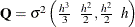
-
order-3 spline:
 ,
, 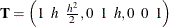 , and
, and
![\[ \mb {Q}[i, j] = \sigma ^{2}* \frac{h^{6-i-j+1}}{(6-i-j+1)(3-i)! (3-j)! } \; \; 1 \leq i, j \leq 3 \]](images/etsug_ssm0334.png)
Decay and Growth Trends
There are two choices for the decay trend: DECAY and DECAY(OU). Similarly, there are two choices for the growth trend: GROWTH and GROWTH(OU). The “OU” stands for the Ornstein-Uhlenbeck form of these models. The decay trend is a sum of two correlated components: one component is a random walk, and the other component is a stationary autoregression. In its Ornstein-Uhlenbeck form, the random walk component is replaced by a constant. The growth trend (and its Ornstein-Uhlenbeck variant) has the same form as the decay trend except that the autorgression is nonstationary (in fact, it is explosive). For growth trend models, floating-point errors can result for even moderately long forecast horizons because of the explosive growth in the trend values.
The system matrices for the decay and the growth types in their respective cases are identical, except for the sign of the
rate parameter ![]() :
: ![]() for the decay type, and
for the decay type, and ![]() for the growth type. In addition, the initial conditions for the growth models are fully diffuse; they are only partially
diffuse for the decay models. The underlying state vector for all these models is two-dimensional.
for the growth type. In addition, the initial conditions for the growth models are fully diffuse; they are only partially
diffuse for the decay models. The underlying state vector for all these models is two-dimensional.
The system matrices for the DECAY type are:
|
|
|
|
|
|
|
|
|
|
|
|
The initial condition is partially diffuse with ![]() . The system matrices for the GROWTH type are the same (with
. The system matrices for the GROWTH type are the same (with ![]() ), except that the initial condition is fully diffuse; so
), except that the initial condition is fully diffuse; so ![]() .
.
For the DECAY(OU) type, ![]() and
and ![]() are the same as DECAY, whereas
are the same as DECAY, whereas
|
|
The system matrices for the GROWTH(OU) type are the same (with ![]() ), except that the initial condition is fully diffuse; so
), except that the initial condition is fully diffuse; so ![]() .
.