The TCOUNTREG Procedure (Experimental)
- Overview
- Getting Started
-
Syntax

-
DetailsSpecification of RegressorsMissing ValuesPoisson RegressionNegative Binomial RegressionZero-Inflated Count Regression OverviewZero-Inflated Poisson RegressionZero-Inflated Negative Binomial RegressionVariable SelectionPanel Data AnalysisComputational ResourcesNonlinear Optimization OptionsCovariance Matrix TypesDisplayed OutputOUTPUT OUT= Data SetOUTEST= Data SetODS Table NamesODS Graphics
-
Examples
- References
Panel Data Analysis
Panel Data Poisson Regression with Fixed Effects
The count regression model for panel data can be derived from the Poisson regression model. Consider the multiplicative one-way panel data model,
|
|
where
|
|
Here, ![]() are the individual effects.
are the individual effects.
In the fixed effects model, the ![]() are unknown parameters. The fixed effects model can be estimated by eliminating
are unknown parameters. The fixed effects model can be estimated by eliminating ![]() by conditioning on
by conditioning on ![]() .
.
In the random effects model, the ![]() are independent and identically distributed (iid) random variables, in contrast to the fixed effects model. The random effects
model can then be estimated by assuming a distribution for
are independent and identically distributed (iid) random variables, in contrast to the fixed effects model. The random effects
model can then be estimated by assuming a distribution for ![]() .
.
In the Poisson fixed effects model, conditional on ![]() and parameter
and parameter ![]() ,
, ![]() is iid Poisson distributed with parameter
is iid Poisson distributed with parameter ![]() , and
, and ![]() does not include an intercept. Then, the conditional joint density for the outcomes within the
does not include an intercept. Then, the conditional joint density for the outcomes within the ![]() th panel is
th panel is
|
|
|
|
|
|
|
|
Since ![]() is iid Poisson(
is iid Poisson(![]() ),
), ![]() is the product of
is the product of ![]() Poisson densities. Also,
Poisson densities. Also, ![]() is Poisson(
is Poisson(![]() ). Then,
). Then,
|
|
|
 |
|
|
|
 |
|
|
|
|
|
|
|
|
Thus, the conditional log-likelihood function of the fixed effects Poisson model is given by
|
|
The gradient is
|
|
|
|
|
|
|
|
where
|
|
Panel Data Poisson Regression with Random Effects
In the Poisson random effects model, conditional on ![]() and parameter
and parameter ![]() ,
, ![]() is iid Poisson distributed with parameter
is iid Poisson distributed with parameter ![]() , and the individual effects,
, and the individual effects, ![]() , are assumed to be iid random variables. The joint density for observations in all time periods for the
, are assumed to be iid random variables. The joint density for observations in all time periods for the ![]() th individual,
th individual, ![]() , can be obtained after the density
, can be obtained after the density ![]() of
of ![]() is specified.
is specified.
Let
|
|
so that ![]() and
and ![]() :
:
|
|
Let ![]() . Since
. Since ![]() is conditional on
is conditional on ![]() and parameter
and parameter ![]() is iid Poisson(
is iid Poisson(![]() ), the conditional joint probability for observations in all time periods for the
), the conditional joint probability for observations in all time periods for the ![]() th individual,
th individual, ![]() , is the product of
, is the product of ![]() Poisson densities:
Poisson densities:
|
|
|
|
|
|
|
|
|
|
|
|
|
|
|
|
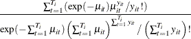
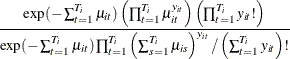
Then, the joint density for the ![]() th panel conditional on just the
th panel conditional on just the ![]() can be obtained by integrating out
can be obtained by integrating out ![]() :
:
|
|
|
|
|
|
|
|
|
|
|
|
|
|
|
|
|
|
|
|
|
|
|
|
|
|
|
|
where ![]() is the overdispersion parameter. This is the density of the Poisson random effects model with gamma-distributed random effects.
For this distribution,
is the overdispersion parameter. This is the density of the Poisson random effects model with gamma-distributed random effects.
For this distribution, ![]() and
and ![]() ; that is, there is overdispersion.
; that is, there is overdispersion.
Then the log-likelihood function is written as
|
|
|
|
|
|
|
|
|
|
|
|
The gradient is
|
|
|
|
|
|
|
|
|
|
|
|
and
|
|
|
|
|
|
|
|
where ![]() ,
, ![]() and
and ![]() is the digamma function.
is the digamma function.
Panel Data Negative Binomial Regression with Fixed Effects
This section shows the derivation of a negative binomial model with fixed effects. Keep the assumptions of the Poisson-distributed dependent variable
|
|
But now let the Poisson parameter be random with gamma distribution and parameters ![]() ,
,
|
|
where one of the parameters is the exponentially affine function of independent variables ![]() . Use integration by parts to obtain the distribution of
. Use integration by parts to obtain the distribution of ![]() ,
,
|
|
|
|
|
|
|
|
which is a negative binomial distribution with parameters ![]() . Conditional joint distribution is given as
. Conditional joint distribution is given as
|
|
|
|
|
|
|
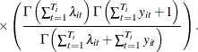 |
Hence, the conditional fixed-effects negative binomial log-likelihood is
|
|
|
|
|
|
|
|
The gradient is
|
|
|
![$\displaystyle \sum _{i=1}^{N}\left[\left(\frac{\Gamma \left(\sum _{t=1}^{T_{i}}\lambda _{it}\right)}{\Gamma \left(\sum _{t=1}^{T_{i}}\lambda _{it}\right)}-\frac{\Gamma \left(\sum _{t=1}^{T_{i}}\lambda _{it}+\sum _{t=1}^{T_{i}}y_{it}\right)}{\Gamma \left(\sum _{t=1}^{T_{i}}\lambda _{it}+\sum _{t=1}^{T_{i}}y_{it}\right)}\right)\sum _{t=1}^{T_{i}}\lambda _{it}\mathbf{x}_{it}\right] $](images/etsug_tcountreg0341.png) |
|
|
|
 |
|
|
|
|
Panel Data Negative Binomial Regression with Random Effects
This section describes the derivation of negative binomial model with random effects. Suppose
|
|
with the Poisson parameter distributed as gamma,
|
|
where its parameters are also random:
|
|
Assume that the distribution of a function of ![]() is beta with parameters
is beta with parameters ![]() :
:
|
|
Explicitly, the beta density with ![]() domain is
domain is
|
|
where ![]() is the beta function. Then, conditional joint distribution of dependent variables is
is the beta function. Then, conditional joint distribution of dependent variables is
|
|
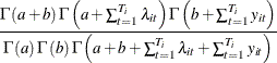
Integrating out the variable ![]() yields the following conditional distribution function:
yields the following conditional distribution function:
|
|
|
|
|
|
|
 |
|
|
|
|
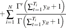
Consequently, the conditional log-likelihood function for a negative binomial model with random effects is
|
|
|
|
|
|
|
|
|
|
|
|
The gradient is
|
|
|
![$\displaystyle \sum _{i=1}^{N}\left[\frac{\Gamma \left(a+\sum _{t=1}^{T_{i}}\lambda _{it}\right)}{\Gamma \left(a+\sum _{t=1}^{T_{i}}\lambda _{it}\right)}\sum _{t=1}^{T_{i}}\lambda _{it}\mathbf{x}_{it}+\frac{\Gamma \left(b+\sum _{t=1}^{T_{i}}y_{it}\right)}{\Gamma \left(b+\sum _{t=1}^{T_{i}}y_{it}\right)}\right] $](images/etsug_tcountreg0362.png) |
|
|
|
![$\displaystyle -\sum _{i=1}^{N}\left[\frac{\Gamma \left(a+b+\sum _{t=1}^{T_{i}}\lambda _{it}+\sum _{t=1}^{T_{i}}y_{it}\right)}{\Gamma \left(a+b+\sum _{t=1}^{T_{i}}\lambda _{it}+\sum _{t=1}^{T_{i}}y_{it}\right)}\sum _{t=1}^{T_{i}}\lambda _{it}\mathbf{x}_{it}\right] $](images/etsug_tcountreg0363.png) |
|
|
|
|
and
|
|
|
![$\displaystyle \sum _{i=1}^{N}\left[\frac{\Gamma \left(a+b\right)}{\Gamma \left(a+b\right)}+\frac{\Gamma \left(a+\sum _{t=1}^{T_{i}}\lambda _{it}\right)}{\Gamma \left(a+\sum _{t=1}^{T_{i}}\lambda _{it}\right)}\right] $](images/etsug_tcountreg0367.png) |
|
|
|
![$\displaystyle -\sum _{i=1}^{N}\left[\frac{\Gamma \left(a\right)}{\Gamma \left(a\right)}+\frac{\Gamma \left(a+b+\sum _{t=1}^{T_{i}}\lambda _{it}+\sum _{t=1}^{T_{i}}y_{it}\right)}{\Gamma \left(a+b+\sum _{t=1}^{T_{i}}\lambda _{it}+\sum _{t=1}^{T_{i}}y_{it}\right)}\right], $](images/etsug_tcountreg0368.png) |
and
|
|
|
![$\displaystyle \sum _{i=1}^{N}\left[\frac{\Gamma \left(a+b\right)}{\Gamma \left(a+b\right)}+\frac{\Gamma \left(b+\sum _{t=1}^{T_{i}}y_{it}\right)}{\Gamma \left(b+\sum _{t=1}^{T_{i}}y_{it}\right)}\right] $](images/etsug_tcountreg0371.png) |
|
|
|
![$\displaystyle -\sum _{i=1}^{N}\left[\frac{\Gamma \left(b\right)}{\Gamma \left(b\right)}+\frac{\Gamma \left(a+b+\sum _{t=1}^{T_{i}}\lambda _{it}+\sum _{t=1}^{T_{i}}y_{it}\right)}{\Gamma \left(a+b+\sum _{t=1}^{T_{i}}\lambda _{it}+\sum _{t=1}^{T_{i}}y_{it}\right)}\right]. $](images/etsug_tcountreg0372.png) |