The ARIMA Procedure
- Overview
-
Getting Started
 The Three Stages of ARIMA ModelingIdentification StageEstimation and Diagnostic Checking StageForecasting StageUsing ARIMA Procedure StatementsGeneral Notation for ARIMA ModelsStationarityDifferencingSubset, Seasonal, and Factored ARMA ModelsInput Variables and Regression with ARMA ErrorsIntervention Models and Interrupted Time SeriesRational Transfer Functions and Distributed Lag ModelsForecasting with Input VariablesData Requirements
 -
Syntax

-
Details
 The Inverse Autocorrelation FunctionThe Partial Autocorrelation FunctionThe Cross-Correlation FunctionThe ESACF MethodThe MINIC MethodThe SCAN MethodStationarity TestsPrewhiteningIdentifying Transfer Function ModelsMissing Values and AutocorrelationsEstimation DetailsSpecifying Inputs and Transfer FunctionsInitial ValuesStationarity and InvertibilityNaming of Model ParametersMissing Values and Estimation and ForecastingForecasting DetailsForecasting Log Transformed DataSpecifying Series PeriodicityDetecting OutliersOUT= Data SetOUTCOV= Data SetOUTEST= Data SetOUTMODEL= SAS Data SetOUTSTAT= Data SetPrinted OutputODS Table NamesStatistical Graphics
 -
Examples

- References
This example illustrates the ARIMA procedure results for a case where the true model is known. An integrated moving-average model is used for this illustration.
The following DATA step generates a pseudo-random sample of 100 periods from the ARIMA(0,1,1) process ![]() ,
, ![]() :
:
title1 'Simulated IMA(1,1) Series';
data a;
  u1 = 0.9; a1 = 0;
  do i = -50 to 100;
     a = rannor( 32565 );
     u = u1 + a - .8 * a1;
     if i > 0 then output;
     a1 = a;
     u1 = u;
  end;
run;
The following ARIMA procedure statements identify and estimate the model:
/*-- Simulated IMA Model --*/
proc arima data=a;
  identify var=u;
  run;
  identify var=u(1);
  run;
  estimate q=1 ;
  run;
quit;
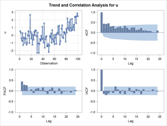
The graphical series correlation analysis output of the first IDENTIFY statement is shown in Output 7.1.1. The output shows the behavior of the sample autocorrelation function when the process is nonstationary. Note that in this case the estimated autocorrelations are not very high, even at small lags. Nonstationarity is reflected in a pattern of significant autocorrelations that do not decline quickly with increasing lag, not in the size of the autocorrelations.
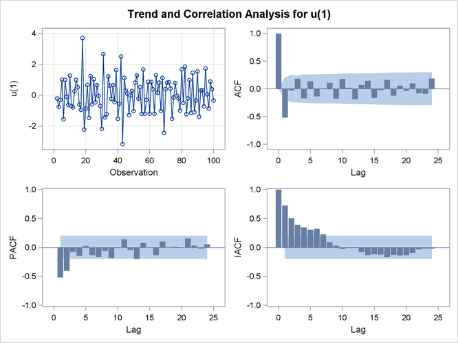
The second IDENTIFY statement differences the series. The results of the second IDENTIFY statement are shown in Output 7.1.2. This output shows autocorrelation, inverse autocorrelation, and partial autocorrelation functions typical of MA(1) processes.
The ESTIMATE statement fits an ARIMA(0,1,1) model to the simulated data. Note that in this case the parameter estimates are
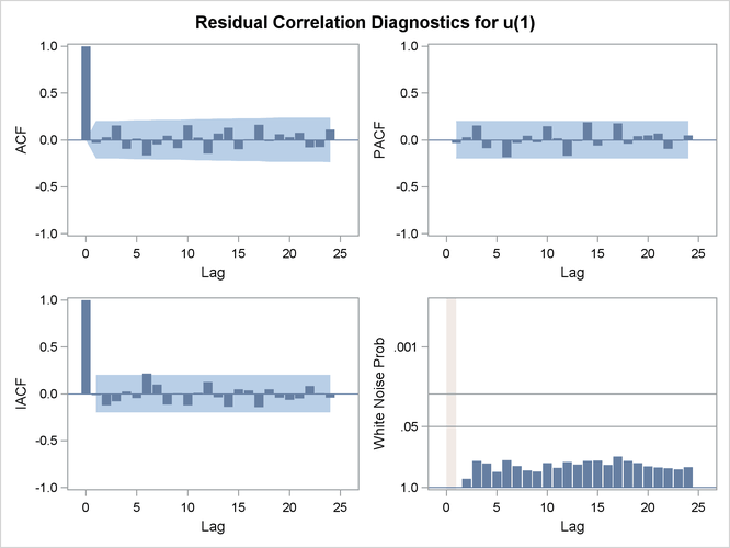
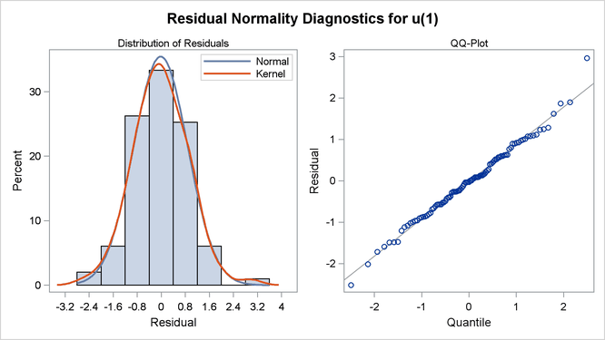
reasonably close to the values used to generate the simulated data. (![]() ) Moreover, the graphical analysis of the residuals shows no model inadequacies (see Output 7.1.4 and Output 7.1.5).
) Moreover, the graphical analysis of the residuals shows no model inadequacies (see Output 7.1.4 and Output 7.1.5).
The ESTIMATE statement results are shown in Output 7.1.3.
Output 7.1.3: Output from Fitting ARIMA(0,1,1) Model
| Conditional Least Squares Estimation | |||||
|---|---|---|---|---|---|
| Parameter | Estimate | Standard Error | t Value | Approx Pr > |t| |
Lag |
| MU | 0.02056 | 0.01972 | 1.04 | 0.2997 | 0 |
| MA1,1 | 0.79142 | 0.06474 | 12.22 | <.0001 | 1 |
| Constant Estimate | 0.020558 |
|---|---|
| Variance Estimate | 0.819807 |
| Std Error Estimate | 0.905432 |
| AIC | 263.2594 |
| SBC | 268.4497 |
| Number of Residuals | 99 |
| Model for variable u | |
|---|---|
| Estimated Mean | 0.020558 |
| Period(s) of Differencing | 1 |
| Moving Average Factors | |
|---|---|
| Factor 1: | 1 - 0.79142 B**(1) |


