The PANEL Procedure

Da Silva Method (Variance-Component Moving Average Model)

The Da Silva method assumes that the observed value of the dependent variable at the tth time point on the ith cross-sectional unit can be expressed as

$y_{it}= \mb {x} _{it}^{}{\beta } + a_{i}+ b_{t}+ e_{it} \hspace{.3 in} i=1, {\ldots }, \mi {N} ;t=1, {\ldots }, \mi {T}$

where

: ${ \mb {x} _{it}^{}=( x_{it1}, {\ldots }, x_{itp})}$ is a vector of explanatory variables for the tth time point and ith cross-sectional unit
: ${{\beta }=( {\beta }_{1}, {\ldots } , {\beta }_{p}{)’}}$ is the vector of parameters
: ${a_{i}}$ is a time-invariant, cross-sectional unit effect
: ${b_{t}}$ is a cross-sectionally invariant time effect
: ${e_{it}}$ is a residual effect unaccounted for by the explanatory variables and the specific time and cross-sectional unit effects

Since the observations are arranged first by cross sections, then by time periods within cross sections, these equations can be written in matrix notation as

$\mb {y} =\mb {X} {\beta }+\mb {u}$

where

$\mb {u} =(\mb {a} {\otimes }\mb {1} _{T})+(\mb {1} _{N}{\otimes }\mb {b} )+\mb {e}$

$\mb {y} = (y_{11},{\ldots },y_{1T}, y_{21},{\ldots },y_{NT}{)’}$

$\mb {X} =(\mb {x} _{11},{\ldots },\mb {x} _{1T},\mb {x} _{21},{\ldots } ,\mb {x} _{NT}{)’}$

$\mb {a} =(a_{1}{\ldots }a_{N}{)’}$

$\mb {b} =(b_{1}{\ldots }b_{T}{)’}$

$\mb {e} = (e_{11},{\ldots },e_{1T}, e_{21},{\ldots },e_{NT}{)’}$

Here 1 $_{N}$ is an ${\mi {N} \times 1}$ vector with all elements equal to 1, and ${\otimes }$ denotes the Kronecker product.

The following conditions are assumed:

${ \mb {x} _{it}}$ is a sequence of nonstochastic, known ${p{\times }1}$ vectors in ${ {\Re }^{p}}$ whose elements are uniformly bounded in ${ {\Re }^{p}}$ . The matrix X has a full column rank p.
$\bbeta$ is a ${p \times 1}$ constant vector of unknown parameters.
a is a vector of uncorrelated random variables such that ${{E}( a_{i})=0}$ and ${\mr {var}( a_{i})= {\sigma }^{2}_{a}}$ , ${ {\sigma }^{2}_{a}>0, i=1, {\ldots }, \mi {N} }$ .
b is a vector of uncorrelated random variables such that ${{E}( b_{t})=0}$ and $\mr {var}( b_{t})= {\sigma }^{2}_{b}$ where ${\sigma }^{2}_{b}>0$ and $t=1, {\ldots }, \mi {T}$ .
${ \mb {e} _{i}=( e_{i1},{\ldots },e_{iT}{)’}}$ is a sample of a realization of a finite moving-average time series of order ${m < \mi {T} -1}$ for each i ; hence,

$e_{it}={\alpha }_{0} {\epsilon }_{it}+ {\alpha }_{1} {\epsilon }_{it-1}+{\ldots }+ {\alpha }_{m} {\epsilon }_{it-m} \; \; \; \; t=1,{\ldots },\mi {T} ; i=1,{\ldots },\mi {N}$

where ${{\alpha }_{0}, {\alpha }_{1},{\ldots }, {\alpha }_{m}}$ are unknown constants such that ${\alpha }_{0}{\ne }0$ and ${{\alpha }_{m}{\ne }0}$ , and ${ \{ {\epsilon }_{ij}\} ^{j={\infty }}_{j=-{\infty }}}$ is a white noise process for each $i$ —that is, a sequence of uncorrelated random variables with ${{E}( {\epsilon }_{t})=0,{E}( {\epsilon }^{2}_{t})= {\sigma }^{2}_{{\epsilon }} }$ , and ${ {\sigma }^{2}_{{\epsilon }}>0 }$ . ${ \{ {\epsilon }_{ij}\} ^{j={\infty }}_{j=-{\infty }}}$ for ${i=1, {\ldots }, \mi {N} }$ are mutually uncorrelated.
The sets of random variables ${ \{ a_{i}\} ^{N}_{i=1}}$ , ${ \{ b_{t}\} ^{T}_{t=1}}$ , and ${ \{ e_{it}\} ^{T}_{t=1}}$ for ${i=1, {\ldots }, \mi {N} }$ are mutually uncorrelated.
The random terms have normal distributions ${ a_{i}{\sim }{N}(0, {\sigma }^{2}_{a}), b_{t}{\sim }{N}(0, {\sigma }^{2}_{b}), }$ and ${ {\epsilon }_{t-k}{\sim }{N}(0, {\sigma }^{2}_{{\epsilon }}), }$ for ${i=1, {\ldots }, \mi {N} ; t=1,{\ldots } \mi {T} ;}$ and $k=1, {\ldots }, m$ .

If assumptions 1–6 are satisfied, then

${E}(\mb {y} )=\mb {X} {\beta }$

and

$\mr {var}(\mb {y} )= {\sigma }^{2}_{a} (I_{N}{\otimes }J_{T})+ {\sigma }^{2}_{b}(J_{N}{\otimes }I_{T})+ (I_{N}{\otimes }{\Psi }_{T})$

where ${{\Psi }_{T}}$ is a ${\mi {T} \times \mi {T} }$ matrix with elements ${{\psi }_{ts}}$ as follows:

$\mr {Cov}( e_{it} e_{is})= \begin{cases} {\psi }({|t-s|}) & \mr {if}\hspace{.1 in} {|t-s|} {\le } m \\ 0 & \mr {if} \hspace{.1 in}{|t-s|} > m \end{cases}$

where ${{\psi }(k) = {\sigma }^{2}_{{\epsilon }}\sum _{j=0}^{m-k}{{\alpha }_{j}{\alpha }_{j+k}}}$ for ${k={|t-s|}}$ . For the definition of ${I_{N}}$ , ${I_{T}}$ , ${J_{N}}$ , and ${J_{T}}$ , see the section Fuller and Battese’s Method.

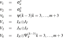
The covariance matrix, denoted by V, can be written in the form

$\mb {V} = {\sigma }^{2}_{a}(I_{N}{\otimes }J_{T}) + {\sigma }^{2}_{b}(J_{N}{\otimes }I_{T}) +\sum _{k=0}^{m}{{\psi }(k)(I_{N}{\otimes } {\Psi }^{(k)}_{T})}$

where ${ {\Psi }^{(0)}_{T}=I_{T}}$ , and, for k =1, ${\ldots }$ , m, ${ {\Psi }^{(k)}_{T}}$ is a band matrix whose kth off-diagonal elements are 1’s and all other elements are 0’s.

Thus, the covariance matrix of the vector of observations y has the form

${\mr {Var}}(\mb {y} )=\sum _{k=1}^{m+3}{{\nu }_{k}V_{k}}$

where

$\begin{eqnarray*} {\nu }_{1}& =& {\sigma }^{2}_{a} \\ {\nu }_{2}& =& {\sigma }^{2}_{b} \\ {\nu }_{k}& =& {\psi }(k-3) k=3,{\ldots }, m+3 \\ V_{1}& =& I_{N}{\otimes }J_{T} \\ V_{2}& =& J_{N}{\otimes }I_{T} \\ V_{k}& =& I_{N}{\otimes } {\Psi }^{(k-3)}_{T} k=3,{\ldots }, m+3 \nonumber \end{eqnarray*}$

The estimator of $\bbeta$ is a two-step GLS-type estimator—that is, GLS with the unknown covariance matrix replaced by a suitable estimator of V. It is obtained by substituting Seely estimates for the scalar multiples ${{\nu }_{k},k=1, 2, {\ldots }, m+3}$ .

Seely (1969) presents a general theory of unbiased estimation when the choice of estimators is restricted to finite dimensional vector spaces, with a special emphasis on quadratic estimation of functions of the form ${\sum _{i=1}^{n}{{\delta }_{i}{\nu }_{i}}}$ .

The parameters ${{\nu }_{i}}$ (i =1, ${\ldots }$ , n) are associated with a linear model E(y )=X ${\beta }$ with covariance matrix ${\sum _{i=1}^{n}{{\nu }_{i}V_{i}}}$ where ${V_{i}}$ (i =1, ${\ldots }$ , n) are real symmetric matrices. The method is also discussed by Seely (1970b, 1970a); Seely and Zyskind (1971). Seely and Soong (1971) consider the MINQUE principle, using an approach along the lines of Seely (1969).