The QLIM Procedure
- Overview
-
Getting Started

-
Syntax

-
Details
 Ordinal Discrete Choice ModelingLimited Dependent Variable ModelsStochastic Frontier Production and Cost ModelsHeteroscedasticity and Box-Cox TransformationBivariate Limited Dependent Variable ModelingSelection ModelsMultivariate Limited Dependent ModelsVariable SelectionTests on ParametersEndogeneity and Instrumental VariablesBayesian AnalysisPrior DistributionsOutput to SAS Data SetOUTEST= Data SetNamingODS Table NamesODS Graphics
 -
Examples

- References
This example illustrates how to use the QLIM procedure to perform Bayesian analysis. The generated data mimic a hypothetical scenario in which you study the number of tickets sold for a sports event given the probability of the hosting team winning and the price of the tickets. The following statements create the dataset:
title1 'Bayesian Analysis';

ods graphics on;

data test;
   do i=1 to 200;
      e1 = rannor(8726)*2000;
      WinChance = ranuni(8772);
      Price = 10+ranexp(8773)*4;
      y = 48000 + 5000*WinChance - 100 * price +  e1;
      if y>50000 then TicketSales = 50000;
      if y<=50000 then TicketSales = y;
      output;
   end;
   keep WinChance price  y TicketSales;
run;
The following statements perform Bayesian analysis of a Tobit model:
proc qlim data=test plots(prior)=all;
   model TicketSales = WinChance price;
   endogenous TicketSales ~ censored(lb=0 ub= 50000);
   prior intercept~normal(mean=48000);
   prior WinChance~normal(mean=5000);
   prior Price~normal(mean=-100);
   bayes NBI=10000 NMC=30000 THIN=1 ntrds=1 DIAG=ALL STATS=ALL seed=2;
run;
Output 22.8.1 shows the results from the maximum likelihood estimation and the Bayesian analysis with diffuse prior of this Tobit model.
Output 22.8.1: Bayesian Tobit Model
| Bayesian Analysis |
| Parameter Estimates | |||||
|---|---|---|---|---|---|
| Parameter | DF | Estimate | Standard Error | t Value | Approx Pr > |t| |
| Intercept | 1 | 48119 | 623.565045 | 77.17 | <.0001 |
| WinChance | 1 | 5242.083501 | 559.151222 | 9.38 | <.0001 |
| Price | 1 | -106.731665 | 40.660795 | -2.62 | 0.0087 |
| _Sigma | 1 | 1939.607206 | 134.348772 | 14.44 | <.0001 |
| Posterior Summaries | ||||||
|---|---|---|---|---|---|---|
| Parameter | N | Mean | Standard Deviation |
Percentiles | ||
| 25% | 50% | 75% | ||||
| Intercept | 30000 | 48109.4 | 535.0 | 47750.5 | 48102.6 | 48460.1 |
| WinChance | 30000 | 5212.9 | 483.4 | 4878.8 | 5205.2 | 5533.0 |
| Price | 30000 | -104.7 | 36.5224 | -128.6 | -104.2 | -79.4191 |
| _Sigma | 30000 | 1950.9 | 132.9 | 1858.4 | 1945.0 | 2034.0 |
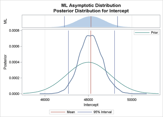
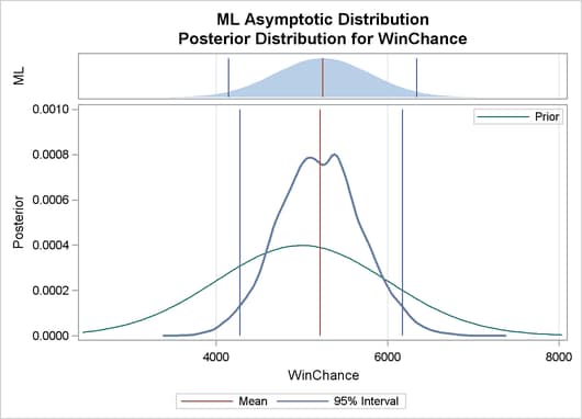
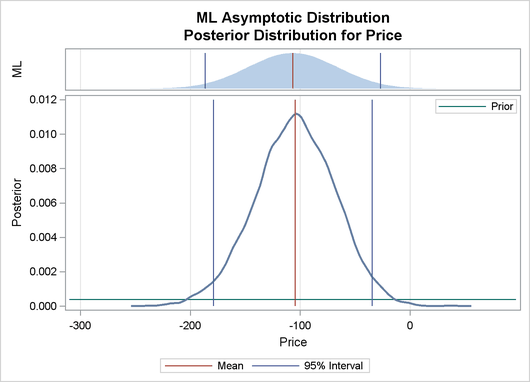
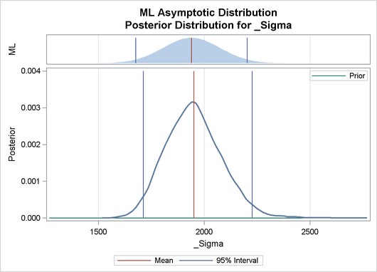
Output 22.8.2 depicts a graphical representation of MLE, prior, and posterior distributions.
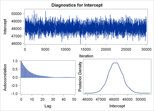
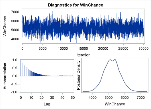
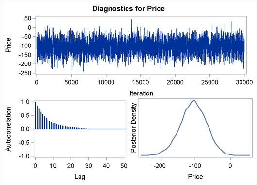
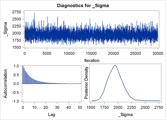
The validity of the MCMC sampling phase can be monitored with Output 22.8.3.
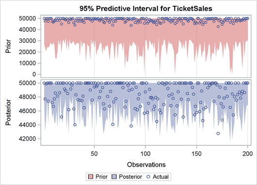
Finally the prior and the posterior predictive analyses are represented in Output 22.8.4
