Creating Standard Deviation Charts from Raw Data

Note: See Standard Deviation Chart (s Chart) Example in the SAS/QC Sample Library.

A petroleum company uses a turbine to heat water into steam, which is then pumped into the ground to make oil less viscous and easier to extract. This heating process occurs 20 times daily, and the amount of power (in kilowatts) used to heat the water to the desired temperature is recorded. The following statements create a SAS data set named Turbine, which contains the power output measurements for 20 days:

data Turbine;
   informat Day date7.;
   format Day date5.;
   input Day @;
   do i=1 to 10;
      input KWatts @;
      output;
   end;
   drop i;
   datalines;
 04JUL94 3196 3507 4050 3215 3583 3617 3789 3180 3505 3454
 04JUL94 3417 3199 3613 3384 3475 3316 3556 3607 3364 3721
 05JUL94 3390 3562 3413 3193 3635 3179 3348 3199 3413 3562
 05JUL94 3428 3320 3745 3426 3849 3256 3841 3575 3752 3347
 06JUL94 3478 3465 3445 3383 3684 3304 3398 3578 3348 3369
 06JUL94 3670 3614 3307 3595 3448 3304 3385 3499 3781 3711
 07JUL94 3448 3045 3446 3620 3466 3533 3590 3070 3499 3457

   ... more lines ...   

 22JUL94 3415 3445 3561 3494 3140 3090 3561 3800 3056 3536
 23JUL94 3421 3787 3454 3699 3307 3917 3292 3310 3283 3536
 23JUL94 3756 3145 3571 3331 3725 3605 3547 3421 3257 3574
;

A partial listing of Turbine is shown in Figure 17.77.

Figure 17.77: Partial Listing of the Data Set Turbine

Kilowatt Power Output Data

Obs	Day	KWatts
1	04JUL	3196
2	04JUL	3507
3	04JUL	4050
4	04JUL	3215
5	04JUL	3583
6	04JUL	3617
7	04JUL	3789
8	04JUL	3180
9	04JUL	3505
10	04JUL	3454
11	04JUL	3417
12	04JUL	3199
13	04JUL	3613
14	04JUL	3384
15	04JUL	3475
16	04JUL	3316
17	04JUL	3556
18	04JUL	3607
19	04JUL	3364
20	04JUL	3721
21	05JUL	3390
22	05JUL	3562
23	05JUL	3413
24	05JUL	3193
25	05JUL	3635

The data set Turbine is said to be in “strung-out” form, since each observation contains the day and power output for a single heating. The first 20 observations contain the power outputs for the first day, the second 20 observations contain the power outputs for the second day, and so on. Because the variable Day classifies the observations into rational subgroups, it is referred to as the subgroup-variable. The variable KWatts contains the power output measurements and is referred to as the process variable (or process for short).

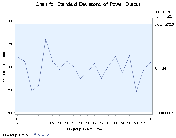
You can use an s chart to determine whether the variability in the heating process is in control. The following statements create the s chart shown in Figure 17.78:

ods graphics off;
symbol v=dot h=.8;
title 'Chart for Standard Deviations of Power Output';
proc shewhart data=Turbine;
   schart KWatts*Day;
run;

This example illustrates the basic form of the SCHART statement. After the keyword SCHART, you specify the process to analyze (in this case, KWatts), followed by an asterisk and the subgroup-variable (Day).

The input data set is specified with the DATA= option in the PROC SHEWHART statement.

Figure 17.78: s Chart for Power Output Data (Traditional Graphics)

Each point on the chart represents the standard deviation of the measurements for a particular day. For instance, the standard deviation plotted for the first day is

$\sqrt { \frac{(3196-3487.4)^{2} + (3507-3487.4)^{2} + \cdots + (3721-3487.4)^{2}}{19}} = 220.26$

Since all of the subgroup standard deviations lie within the control limits, you can conclude that the variability of the process is in statistical control.

By default, the control limits shown are $3\sigma$ limits estimated from the data; the formulas for the limits are given in Table 17.54. You can also read control limits from an input data set; see Reading Preestablished Control Limits.

For computational details, see Constructing Charts for Standard Deviations. For more details on reading raw data, see DATA= Data Set.

SCHART Statement: SHEWHART Procedure

Creating Standard Deviation Charts from Raw Data