Example 52.3 Changing the Bandwidth (Bivariate) :: SAS/STAT(R) 13.1 User's Guide

Example 52.3 Changing the Bandwidth (Bivariate)

Subsections:

Multiple Bandwidths

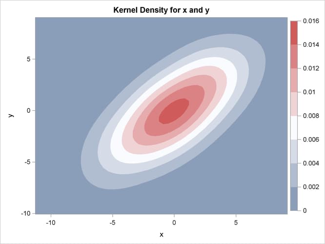
Recall the analysis from the section Getting Started: KDE Procedure. Suppose you would like a slightly smoother estimate. You could then rerun the analysis with a larger bandwidth:

ods graphics on;
proc kde data=bivnormal;
   bivar x y / bwm=2;
run;

The BWM= option requests bandwidth multipliers of 2 for both x and y. With ODS Graphics enabled, the BIVAR statement produces a contour plot, as shown in Output 52.3.1.

Output 52.3.1: Contour Plot of Estimated Density with Additional Smoothing

Multiple Bandwidths

You can also specify multiple bandwidths with only one run of the KDE procedure. Notice that by specifying pairs of variables inside parentheses, a kernel density estimate is computed for each pair. In the following statements the first kernel density is computed with the default bandwidth, but the second kernel density specifies a bandwidth multiplier of 0.5 for the variable x and a multiplier of 2 for the variable y:

proc kde data=bivnormal;
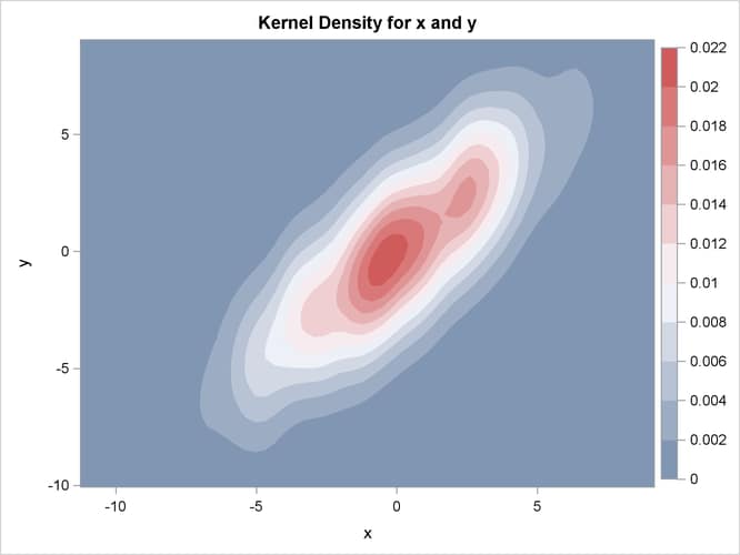
   bivar (x y) (x (bwm=0.5) y (bwm=2));
run;
ods graphics off;

The contour plot of the second kernel density estimate is shown in Output 52.3.2.

Output 52.3.2: Contour Plot of Estimated Density with Different Smoothing for x and y

The KDE Procedure

Example 52.3 Changing the Bandwidth (Bivariate)

Multiple Bandwidths