The GLMPOWER Procedure

The multivariate model has the form
where ![]() is the N
is the N ![]() p vector of responses, for p > 1;
p vector of responses, for p > 1; ![]() is the N
is the N ![]() k design matrix;
k design matrix; ![]() is the k
is the k ![]() p matrix of model parameters that correspond to the columns of
p matrix of model parameters that correspond to the columns of ![]() and
and ![]() ; and
; and ![]() is an N
is an N ![]() p vector of errors, where
p vector of errors, where
In PROC GLMPOWER, the model parameters ![]() are not specified directly, but rather indirectly as
are not specified directly, but rather indirectly as ![]() , which represents either conjectured response means or typical response values for each design profile. The
, which represents either conjectured response means or typical response values for each design profile. The ![]() values are manifested as the collection of dependent variables in the MODEL
statement. The matrix
values are manifested as the collection of dependent variables in the MODEL
statement. The matrix ![]() is obtained from
is obtained from ![]() according to the least squares equation,
according to the least squares equation,
Note that, in general, there is not a one-to-one mapping between ![]() and
and ![]() . Many different scenarios for
. Many different scenarios for ![]() might lead to the same
might lead to the same ![]() . If you specify
. If you specify ![]() with the intention of representing cell means, keep in mind that PROC GLMPOWER allows scenarios that are not valid cell means according to the model that is specified in the MODEL
statement. For example, if
with the intention of representing cell means, keep in mind that PROC GLMPOWER allows scenarios that are not valid cell means according to the model that is specified in the MODEL
statement. For example, if ![]() exhibits an interaction effect but the corresponding interaction term is left out of the model, then the cell means (
exhibits an interaction effect but the corresponding interaction term is left out of the model, then the cell means (![]() ) that are derived from
) that are derived from ![]() differ from
differ from ![]() . In particular, the cell means that are derived in this way are the projection of
. In particular, the cell means that are derived in this way are the projection of ![]() onto the model space.
onto the model space.
It is convenient in power analysis to parameterize the design matrix ![]() in three parts,
in three parts, ![]() , defined as follows:
, defined as follows:
-
The q
 k essence design matrix
  is the collection of unique rows of
  . Its rows are sometimes referred to as "design profiles." Here, q
  N is defined simply as the number of unique rows of .
-
The q
1 weight vector  reveals the relative proportions of design profiles, and
  . Row i of is to be included in the design
  times for every
  times that row j is included. The weights are assumed to be standardized (that is, they sum up to 1).
-
The total sample size is N. This is the number of rows in
. If you gather  copies of the ith row of , for i =
  , then you end up with .
The preceding quantities are derived from PROC GLMPOWER syntax as follows:
It is useful to express the crossproduct matrix ![]() in terms of these three parts,
in terms of these three parts,
because this expression factors out the portion (N) that depends on sample size and the portion (![]() ) that depends only on the design structure.
) that depends only on the design structure.
A general linear hypothesis for the univariate model has the form
where ![]() is an l
is an l ![]() k between-subject contrast matrix with rank
k between-subject contrast matrix with rank ![]() ,
, ![]() is a p
is a p ![]() m within-subject contrast matrix with rank
m within-subject contrast matrix with rank ![]() , and
, and ![]() is an l
is an l ![]() m null contrast matrix (usually just a matrix of zeros).
m null contrast matrix (usually just a matrix of zeros).
Note that model effect tests are just between-subject contrasts that use special forms of ![]() , combined with an
, combined with an ![]() that is the p
that is the p ![]() 1 mean transformation vector of the dependent variables (a vector of values all equal to
1 mean transformation vector of the dependent variables (a vector of values all equal to ![]() ). Thus, this scheme covers both effect tests (which are specified in the MODEL
statement and the EFFECTS=
option in the POWER
statement) and custom between-subject contrasts (which are specified in the CONTRAST
statement).
). Thus, this scheme covers both effect tests (which are specified in the MODEL
statement and the EFFECTS=
option in the POWER
statement) and custom between-subject contrasts (which are specified in the CONTRAST
statement).
The ![]() matrix is often referred to as the dependent variable transformation and is specified in the MANOVA
or REPEATED
statement.
matrix is often referred to as the dependent variable transformation and is specified in the MANOVA
or REPEATED
statement.
The model degrees of freedom ![]() are equal to the rank of
are equal to the rank of ![]() , denoted
, denoted ![]() . The error degrees of freedom
. The error degrees of freedom ![]() are equal to N –
are equal to N – ![]() .
.
The hypothesis sum of squares ![]() in the univariate model generalizes to the hypothesis SSCP matrix in the multivariate model,
in the univariate model generalizes to the hypothesis SSCP matrix in the multivariate model,
The error sum of squares ![]() in the univariate model generalizes to the error SSCP matrix in the multivariate model,
in the univariate model generalizes to the error SSCP matrix in the multivariate model,
where
and
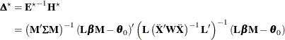
The population counterpart of ![]() is
is
and the population counterpart of ![]() is
is
The elements of ![]() are specified in the MATRIX=
and STDDEV=
options and identified in the CORRMAT=
, CORRS=
, COVMAT=
, and SQRTVAR=
options in the POWER
statement.
are specified in the MATRIX=
and STDDEV=
options and identified in the CORRMAT=
, CORRS=
, COVMAT=
, and SQRTVAR=
options in the POWER
statement.
The power and sample size computations for all the tests that are supported in the MTEST=
option in the POWER
statement are based on ![]() and
and ![]() . The following two subsections cover the computational methods and formulas for the multivariate and univariate tests that
are supported in the MTEST=
and UEPSDEF=
options in the POWER
statement.
. The following two subsections cover the computational methods and formulas for the multivariate and univariate tests that
are supported in the MTEST=
and UEPSDEF=
options in the POWER
statement.
Power computations for multivariate tests are based on O’Brien and Shieh (1992) (for METHOD= OBRIENSHIEH) and Muller and Peterson (1984) (for METHOD= MULLERPETERSON).
Let s = ![]() , the smaller of the between-subject and within-subject contrast degrees of freedom. Critical value computations assume that
under
, the smaller of the between-subject and within-subject contrast degrees of freedom. Critical value computations assume that
under ![]() , the test statistic F is distributed as
, the test statistic F is distributed as ![]() , where
, where ![]() if s = 1 but depends on the choice of test if s > 1. Power computations assume that under
if s = 1 but depends on the choice of test if s > 1. Power computations assume that under ![]() , F is distributed as
, F is distributed as ![]() , where the noncentrality
, where the noncentrality ![]() depends on
depends on ![]() ,
, ![]() , the choice of test, and the power computation method.
, the choice of test, and the power computation method.
Formulas for the test statistic F, denominator degrees of freedom ![]() , and noncentrality
, and noncentrality ![]() for all combinations of dimensions, tests, and methods are given in the following subsections.
for all combinations of dimensions, tests, and methods are given in the following subsections.
The power in each case is computed as
Computed power is exact for some cases and approximate for others. Sample size is computed by inverting the power equation.
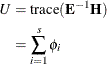
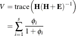
Let ![]() , and define
, and define ![]() as the
as the ![]() vector of ordered positive eigenvalues of
vector of ordered positive eigenvalues of ![]() ,
, ![]() , where
, where ![]() . The population equivalent is
. The population equivalent is
where ![]() is the s
is the s ![]() 1 vector of ordered positive eigenvalues of
1 vector of ordered positive eigenvalues of ![]() ,
, ![]() for
for ![]() .
.
Case 1: s = 1
When s = 1, all three multivariate tests (MTEST=
HLT, MTEST=
PT, and MTEST=
WILKS) are equivalent. The test statistic is F = ![]() , where
, where ![]() .
.
When the dependent variable transformation has a single degree of freedom (![]() ), METHOD=
OBRIENSHIEH and METHOD=
MULLERPETERSON are the same, computing exact power by using noncentrality
), METHOD=
OBRIENSHIEH and METHOD=
MULLERPETERSON are the same, computing exact power by using noncentrality ![]() . The sample size must satisfy
. The sample size must satisfy ![]() .
.
When the dependent variable transformation has more than one degree of freedom but the between-subject contrast has a single
degree of freedom (![]() ), METHOD=
OBRIENSHIEH computes exact power by using noncentrality
), METHOD=
OBRIENSHIEH computes exact power by using noncentrality ![]() , and METHOD=
MULLERPETERSON computes approximate power by using
, and METHOD=
MULLERPETERSON computes approximate power by using
The sample size must satisfy ![]() .
.
Case 2: s > 1
When both the dependent variable transformation and the between-subject contrast have more than one degree of freedom (s > 1), METHOD=
OBRIENSHIEH computes the noncentrality as ![]() , where
, where ![]() is the primary noncentrality. The form of
is the primary noncentrality. The form of ![]() depends on the choice of test statistic.
depends on the choice of test statistic.
METHOD=
MULLERPETERSON computes the noncentrality as ![]() , where
, where ![]() has the same form as
has the same form as ![]() except that
except that ![]() is replaced by
is replaced by
Computed power is approximate for both methods when s > 1.
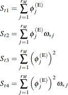
Hotelling-Lawley Trace (MTEST= HLT) When s > 1
If ![]() , then the denominator degrees of freedom for the Hotelling-Lawley trace are
, then the denominator degrees of freedom for the Hotelling-Lawley trace are ![]() ,
,
where
which is the same as ![]() in O’Brien and Shieh (1992) and is due to McKeon (1974).
in O’Brien and Shieh (1992) and is due to McKeon (1974).
If ![]() , then
, then ![]() ,
,
which is the same as both ![]() in O’Brien and Shieh (1992) and
in O’Brien and Shieh (1992) and ![]() in Muller and Peterson (1984) and is due to Pillai and Samson (1959).
in Muller and Peterson (1984) and is due to Pillai and Samson (1959).
The primary noncentrality is
The sample size must satisfy
If ![]() , then the test statistic is
, then the test statistic is
where
and
If ![]() , then the test statistic is
, then the test statistic is
Pillai’s Trace (MTEST= PT) When s > 1
The denominator degrees of freedom for Pillai’s trace are
The primary noncentrality is
![\[ \lambda ^\star = s \left( \frac{\sum _{i=1}^ s \frac{\phi _ i^\star }{1+\phi _ i^\star }}{s - \sum _{i=1}^ s \frac{\phi _ i^\star }{1+\phi _ i^\star }} \right) \]](images/statug_glmpower0150.png)
The sample size must satisfy
The test statistic is
where
Wilks’ Lambda (MTEST= WILKS) When s > 1
The denominator degrees of freedom for Wilks’ lambda are
where
![\begin{equation*} t = \begin{cases} 1 & \text {if } r_ L r_ M \le 3 \\ \left[ \frac{(r_ L r_ M)^2 - 4}{r_ L^2 + r_ M^2 - 5} \right]^\frac {1}{2} & \text {if } r_ L r_ M \ge 4 \end{cases}\end{equation*}](images/statug_glmpower0155.png)
The primary noncentrality is
![\[ \lambda ^\star = t \left[ \left(\prod _{i=1}^ s\left[ (1+\phi _ i^\star )^{-1} \right] \right)^{-\frac{1}{t}} - 1 \right] \]](images/statug_glmpower0156.png)
The sample size must satisfy
The test statistic is
where
![\begin{equation*} \begin{split} \Lambda & = \mr{det}(\mb{E})/\mr{det}(\mb{H} + \mb{E}) \\ & = \prod _{i=1}^ s\left[ (1+\phi _ i)^{-1} \right] \end{split}\end{equation*}](images/statug_glmpower0159.png)
Power computations for univariate tests are based on Muller et al. (2007) and Muller and Barton (1989).
The test statistic is
Critical value computations assume that under ![]() , F is distributed as
, F is distributed as ![]() , where
, where ![]() and
and ![]() depend on the choice of test.
depend on the choice of test.
The four tests for the univariate approach to repeated measures differ in their assumptions about the sphericity ![]() of
of ![]() ,
,
Power computations assume that under ![]() , F is distributed as
, F is distributed as ![]() .
.
Formulas for ![]() and
and ![]() for each test and formulas for
for each test and formulas for ![]() ,
, ![]() , and
, and ![]() are given in the following subsections.
are given in the following subsections.
The power in each case is approximated as
Sample size is computed by inverting the power equation.
The sample size must be large enough to yield ![]() ,
, ![]() ,
, ![]() , and
, and ![]() .
.
Because these univariate tests are biased, the achieved significance level might differ from the nominal significance level.
The actual alpha is computed in the same way as the power, except that the noncentrality parameter ![]() is set to 0.
is set to 0.
Define ![]() as the vector of ordered eigenvalues of
as the vector of ordered eigenvalues of ![]() ,
, ![]() , where
, where ![]() , and define
, and define ![]() as the jth eigenvector of
as the jth eigenvector of ![]() . Critical values and power computations are based on the following intermediate parameters:
. Critical values and power computations are based on the following intermediate parameters:
The degrees of freedom and noncentrality in the noncentral F approximation of the test statistic are computed as follows:
Uncorrected Test
The uncorrected test assumes sphericity ![]() , in which case the null F distribution is exact, with the following degrees of freedom:
, in which case the null F distribution is exact, with the following degrees of freedom:
Greenhouse-Geisser Adjustment (MTEST= UNCORR)
The Greenhouse-Geisser adjustment to the uncorrected test reduces degrees of freedom by the MLE ![]() of the sphericity,
of the sphericity,
An approximation for the expected value of ![]() is used to compute the degrees of freedom for the null F distribution,
is used to compute the degrees of freedom for the null F distribution,
where
Huynh-Feldt Adjustments (MTEST= HF)
The Huynh-Feldt adjustment reduces degrees of freedom by a nearly unbiased estimate ![]() of the sphericity,
of the sphericity,
![\begin{equation*} \tilde{\varepsilon } = \begin{cases} \frac{N r_ M \hat{\varepsilon } - 2}{r_ M \left[ (N - r_ X) - r_ M \hat{\varepsilon } \right]} & \text {if UEPSDEF=HF}\\ \frac{(N-r_ X+1) r_ M \hat{\varepsilon } - 2}{r_ M \left[ (N - r_ X) - r_ M \hat{\varepsilon } \right]} & \text {if UEPSDEF=HFL}\\ \left(\frac{(\nu _ a-2)(\nu _ a-4)}{\nu _ a^2}\right) \left(\frac{(N-r_ X+1) r_ M \hat{\varepsilon } - 2}{r_ M \left[ (N - r_ X) - r_ M \hat{\varepsilon } \right]}\right) & \text {if UEPSDEF=CM} \end{cases}\end{equation*}](images/statug_glmpower0188.png)
where
The value of ![]() is truncated if necessary to be at least
is truncated if necessary to be at least ![]() and at most 1.
and at most 1.
An approximation for the expected value of ![]() is used to compute the degrees of freedom for the null F distribution,
is used to compute the degrees of freedom for the null F distribution,
where
and
![\begin{equation*} \mr{E}(\tilde{\varepsilon }) = \begin{cases} \frac{N \mr{E}(t_1) - 2 \mr{E}(t_2)}{r_ M \left[ (N - r_ X) \mr{E}(t_2) - \mr{E}(t_1) \right]} & \text {if UEPSDEF=HF}\\ \frac{(N-r_ X+1) \mr{E}(t_1) - 2 \mr{E}(t_2)}{r_ M \left[ (N - r_ X) \mr{E}(t_2) - \mr{E}(t_1) \right]} & \text {if UEPSDEF=HFL}\\ \left(\frac{(\nu _ a-2)(\nu _ a-4)}{\nu _ a^2}\right) \left(\frac{(N-r_ X+1) \mr{E}(t_1) - 2 \mr{E}(t_2)}{r_ M \left[ (N - r_ X) \mr{E}(t_2) - \mr{E}(t_1) \right]}\right) & \text {if UEPSDEF=CM} \end{cases}\end{equation*}](images/statug_glmpower0192.png)
Box Conservative Test (MTEST= BOX)
The Box conservative test assumes the worst case for sphericity, ![]() , leading to the following degrees of freedom for the null F distribution:
, leading to the following degrees of freedom for the null F distribution: