The GLMPOWER Procedure
This example demonstrates how to use PROC GLMPOWER to compute and plot power for each effect test in a two-way analysis of variance (ANOVA).
Suppose you are planning an experiment to study the effect of light exposure at three levels on the growth of two varieties
of flowers. The planned data analysis is a two-way ANOVA with flower height (measured at two weeks) as the response and a
model consisting of the effects of light exposure, flower variety, and their interaction. You want to calculate the power
of each effect test for a balanced design with a total of 60 specimens (10 for each combination of exposure and variety) with
![]() = 0.05 for each test.
= 0.05 for each test.
As a first step, create an exemplary data set describing your conjectures about the underlying population means. You believe that the mean flower height for each combination of variety and exposure level (that is, for each design profile, or for each cell in the design) roughly follows Table 47.1.
Table 47.1: Mean Flower Height (in cm) by Variety and Exposure
|
Exposure |
|||
|---|---|---|---|
|
Variety |
1 |
2 |
3 |
|
1 |
14 |
16 |
21 |
|
2 |
10 |
15 |
16 |
The following statements create a data set named Exemplary containing these cell means.
data Exemplary;
   do Variety = 1 to 2;
      do Exposure = 1 to 3;
         input Height @@;
         output;
      end;
   end;
   datalines;
      14 16 21
      10 15 16
;
You also conjecture that the error standard deviation is about 5 cm.
Use the DATA=
option in the PROC GLMPOWER
statement to specify Exemplary as the exemplary data set. Identify the classification variables (Variety and Exposure) by using the CLASS
statement. Specify the model by using the MODEL
statement. Use the POWER
statement to specify power as the result parameter and provide values for the other analysis parameters, error standard deviation
and total sample size. The following SAS statements perform the power analysis:
proc glmpower data=Exemplary;
   class Variety Exposure;
   model Height = Variety | Exposure;
   power
      stddev = 5
      ntotal = 60
      power  = .;
run;
The MODEL
statement defines the full model including both main effects and the interaction. The POWER=
option in the POWER
statement identifies power as the result parameter with a missing value (POWER=
.). The STDDEV=
option specifies an error standard deviation of 5, and the NTOTAL=
option specifies a total sample size of 60. The default value for the ALPHA=
option sets the significance level to ![]() = 0.05.
= 0.05.
Figure 47.1 shows the output.
The power is about 0.72 for the test of the Variety effect. In other words, there is a probability of 0.72 that the test of the Variety effect will produce a significant result (given the assumptions for the means and error standard deviation). The power is
0.96 for the test of the Exposure effect and 0.19 for the interaction test.
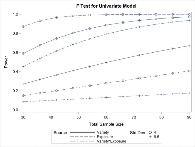
Now, suppose you want to account for some of your uncertainty in conjecturing the true error standard deviation by evaluating the power at reasonable low and high values, 4 and 6.5. You also want to plot power for sample sizes between 30 and 90. The following statements perform the analysis:
ods graphics on;

proc glmpower data=Exemplary;
   class Variety Exposure;
   model Height = Variety | Exposure;
   power
      stddev = 4 6.5
      ntotal = 60
      power  = .;
   plot x=n min=30 max=90;
run;

ods graphics off;
The PLOT statement with the X= N option requests a plot with sample size on the X axis. (The result parameter—in this case, power—is always plotted on the other axis.) The MIN= and MAX= options in the PLOT statement specify the sample size range. The ODS GRAPHICS ON statement enables ODS Graphics.
Figure 47.2 shows the output, and Figure 47.3 shows the plot.
Figure 47.2 reveals that the power ranges from about 0.130 to 0.996 for the different effect tests and scenarios for standard deviation, with a sample size of 60. In Figure 47.3, the line style identifies the effect test, and the plotting symbol identifies the standard deviation. The locations of the plotting symbols identify actual computed powers; the curves are linear interpolations of these points. Note that the computed points in the plot occur at sample size multiples of 6, because there are 6 cells in the design (and by default, sample sizes are rounded to produce integer cell sizes).

