The MI Procedure
- Overview
- Getting Started
-
Syntax

-
Details
 Descriptive StatisticsEM Algorithm for Data with Missing ValuesStatistical Assumptions for Multiple ImputationMissing Data PatternsImputation MethodsMonotone Methods for Data Sets with Monotone Missing PatternsMonotone and FCS Regression MethodsMonotone and FCS Predictive Mean Matching MethodsMonotone and FCS Discriminant Function MethodsMonotone and FCS Logistic Regression MethodsMonotone Propensity Score MethodFCS Methods for Data Sets with Arbitrary Missing PatternsChecking Convergence in FCS MethodsMCMC Method for Arbitrary Missing Multivariate Normal DataProducing Monotone Missingness with the MCMC MethodMCMC Method SpecificationsChecking Convergence in MCMCInput Data SetsOutput Data SetsCombining Inferences from Multiply Imputed Data SetsMultiple Imputation EfficiencyImputer’s Model Versus Analyst’s ModelParameter Simulation versus Multiple ImputationSensitivity Analysis for the MAR AssumptionMultiple Imputation with Pattern-Mixture ModelsSpecifying Sets of Observations for Imputation in Pattern-Mixture ModelsAdjusting Imputed Values in Pattern-Mixture ModelsSummary of Issues in Multiple ImputationODS Table NamesODS Graphics
 -
Examples
 EM Algorithm for MLEMonotone Propensity Score MethodMonotone Regression MethodMonotone Logistic Regression Method for CLASS VariablesMonotone Discriminant Function Method for CLASS VariablesFCS Method for Continuous VariablesFCS Method for CLASS VariablesFCS Method with Trace PlotMCMC MethodProducing Monotone Missingness with MCMCChecking Convergence in MCMCSaving and Using Parameters for MCMCTransforming to NormalityMultistage ImputationCreating Control-Based Pattern Imputation in Sensitivity AnalysisAdjusting Imputed Continuous Values in Sensitivity AnalysisAdjusting Imputed Classification Levels in Sensitivity AnalysisAdjusting Imputed Values with Parameters in a Data Set
 - References
For a data set with an arbitrary missing data pattern, you can use FCS methods to impute missing values for all variables, assuming the existence of a joint distribution for these variables (Brand, 1999; Van Buuren, 2007). FCS method involves two phases in each imputation: the preliminary filled-in phase followed by the imputation phase.
At the filled-in phase, the missing values for all variables are filled in sequentially over the variables taken one at a time. The missing values for each variable are filled in using the specified method, or the default method for the variable if a method is not specified, with preceding variables serving as the covariates. These filled-in values provide starting values for these missing values at the imputation phase.
At the imputation phase, the missing values for each variable are imputed using the specified method and covariates at each iteration. The default method for the variable is used if a method is not specified, and the remaining variables are used as covariates if the set of covariates is not specified. After a number of iterations, as specified with the NBITER= option, the imputed values in each variable are used for the imputation. At each iteration, the missing values are imputed sequentially over the variables taken one at a time.
The MI procedure orders the variables as they are ordered in the VAR statement. For example, if the order of the p variables in the VAR statement is ![]() ,
, ![]() , …,
, …, ![]() , then
, then ![]() ,
, ![]() , …,
, …, ![]() (in that order) are used in the filled-in and imputation phases.
(in that order) are used in the filled-in and imputation phases.
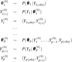
The filled-in phase replaces missing values with filled-in values for each variable. That is, with p variables ![]() ,
, ![]() , …,
, …, ![]() (in that order), the missing values are filled in by using the sequence,
(in that order), the missing values are filled in by using the sequence,

where ![]() is the set of observed
is the set of observed ![]() values,
values, ![]() is the set of filled-in
is the set of filled-in ![]() values,
values, ![]() is the set of both observed and filled-in
is the set of both observed and filled-in ![]() values, and
values, and ![]() is the set of simulated parameters for the conditional distribution of
is the set of simulated parameters for the conditional distribution of ![]() given variables
given variables ![]() ,
, ![]() , …,
, …, ![]() .
.
For each variable ![]() with missing values, the corresponding imputation method is used to fit the model with covariates
with missing values, the corresponding imputation method is used to fit the model with covariates ![]() . The observed observations for
. The observed observations for ![]() , which might include observations with filled-in values for
, which might include observations with filled-in values for ![]() , are used in the model fitting. With this resulting model, a new model is drawn and then used to impute missing values for
, are used in the model fitting. With this resulting model, a new model is drawn and then used to impute missing values for
![]() .
.
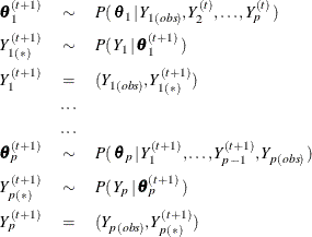
The imputation phase replaces these filled-in values ![]() with imputed values for each variable sequentially at each iteration. That is, with p variables
with imputed values for each variable sequentially at each iteration. That is, with p variables ![]() ,
, ![]() , …,
, …, ![]() (in that order), the missing values are imputed with the sequence at iteration t + 1,
(in that order), the missing values are imputed with the sequence at iteration t + 1,

where ![]() is the set of observed
is the set of observed ![]() values,
values, ![]() is the set of imputed
is the set of imputed ![]() values at iteration t + 1,
values at iteration t + 1, ![]() is the set of filled-in
is the set of filled-in ![]() values (t = 0) or the set of imputed
values (t = 0) or the set of imputed ![]() values at iteration t (t > 0),
values at iteration t (t > 0), ![]() is the set of both observed and imputed
is the set of both observed and imputed ![]() values at iteration t + 1, and
values at iteration t + 1, and ![]() is the set of simulated parameters for the conditional distribution of
is the set of simulated parameters for the conditional distribution of ![]() given covariates constructed from
given covariates constructed from ![]() , …,
, …, ![]() ,
, ![]() , …,
, …, ![]() .
.
At each iteration, a specified model is fitted for each variable with missing values by using observed observations for that variable, which might include observations with imputed values for other variables. With this resulting model, a new model is drawn and then used to impute missing values for the imputed variable.
The steps are iterated long enough for the results to reliably simulate an approximately independent draw of the missing values for an imputed data set.
The imputation methods used in the filled-in and imputation phases are similar to the corresponding monotone methods for monotone missing data. You can use a regression method or a predictive mean matching method to impute missing values for a continuous variable, a logistic regression method for a classification variable with a binary or ordinal response, and a discriminant function method for a classification variable with a binary or nominal response. See the sections Monotone and FCS Regression Methods, Monotone and FCS Predictive Mean Matching Methods, Monotone and FCS Discriminant Function Methods, and Monotone and FCS Logistic Regression Methods for these methods.
The FCS method requires fewer iterations than the MCMC method (Van Buuren, 2007). Often, as few as five or 10 iterations are enough to produce satisfactory results (Van Buuren, 2007; Brand, 1999).