Regression Methods :: SAS/STAT(R) 13.2 User's Guide

Partial Least Squares

Partial least squares (PLS) works by extracting one factor at a time. Let $\mb{X}=\mb{X}_0$ be the centered and scaled matrix of predictors and let $\mb{Y}=\mb{Y}_0$ be the centered and scaled matrix of response values. The PLS method starts with a linear combination $\mb{t} = \mb{X}_0\mb{w}$ of the predictors, where $\mb{t}$ is called a score vector and $\mb{w}$ is its associated weight vector. The PLS method predicts both $\mb{X}_0$ and $\mb{Y}_0$ by regression on $\mb{t}$ :

$\begin{array}{rclcrcl} \hat{\mb{X}}_0 & = & \mb{t} \mb{p}’, & \textrm{where} & \mb{p}’ & = & (\mb{t}’\mb{t} )^{-1}\mb{t}’\mb{X}_0 \\ \hat{\mb{Y}}_0 & = & \mb{t} \mb{c}’, & \textrm{where} & \mb{c}’ & = & (\mb{t}’\mb{t} )^{-1}\mb{t}’\mb{Y}_0 \\ \end{array}$

The vectors $\mb{p}$ and $\mb{c}$ are called the X- and Y-loadings, respectively.

The specific linear combination $\mb{t} = \mb{X}_0\mb{w}$ is the one that has maximum covariance $\mb{t}’\mb{u}$ with some response linear combination $\mb{u} = \mb{Y}_0\mb{q}$ . Another characterization is that the X- and Y-weights $\mb{w}$ and $\mb{q}$ are proportional to the first left and right singular vectors of the covariance matrix $\mb{X}_0’\mb{Y}_0$ or, equivalently, the first eigenvectors of $\mb{X}_0’\mb{Y}^{}_0\mb{Y}_0’\mb{X}^{}_0$ and $\mb{Y}_0’\mb{X}^{}_0\mb{X}_0’\mb{Y}^{}_0$ , respectively.

This accounts for how the first PLS factor is extracted. The second factor is extracted in the same way by replacing $\mb{X}_0$ and $\mb{Y}_0$ with the X- and Y-residuals from the first factor:

$\begin{eqnarray*} \mb{X}_1 & = & \mb{X}_0 - \hat{\mb{X}}_0 \\ \mb{Y}_1 & = & \mb{Y}_0 - \hat{\mb{Y}}_0 \\ \end{eqnarray*}$

These residuals are also called the deflated $\mb{X}$ and $\mb{Y}$ blocks. The process of extracting a score vector and deflating the data matrices is repeated for as many extracted factors as are wanted.

SIMPLS

Note that each extracted PLS factor is defined in terms of different X-variables $\mb{X}_ i$ . This leads to difficulties in comparing different scores, weights, and so forth. The SIMPLS method of De Jong (1993) overcomes these difficulties by computing each score $\mb{t}_ i=\mb{X}\mb{r}_ i$ in terms of the original (centered and scaled) predictors $\mb{X}$ . The SIMPLS X-weight vectors $r_ i$ are similar to the eigenvectors of $\mb{S}\mb{S}’ = \mb{X}’\mb{Y}\mb{Y}’\mb{X}$ , but they satisfy a different orthogonality condition. The $\mb{r}_1$ vector is just the first eigenvector $\mb{e}_1$ (so that the first SIMPLS score is the same as the first PLS score), but whereas the second eigenvector maximizes

$\mb{e}_1’\bS \bS ’\mb{e}_2~ \mbox{subject to}~ \mb{e}_1’\mb{e}_2=0$

the second SIMPLS weight $\mb{r}_2$ maximizes

$\mb{r}_1’SS’\mb{r}_2~ \mbox{subject to}~ \mb{r}_1’\bX ’\bX \mb{r}_2 = \mb{t}_1’\mb{t}_2 = 0$

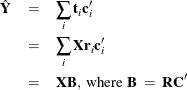
The SIMPLS scores are identical to the PLS scores for one response but slightly different for more than one response; see De Jong (1993) for details. The X- and Y-loadings are defined as in PLS, but since the scores are all defined in terms of $\mb{X}$ , it is easy to compute the overall model coefficients $\mb{B}$ :

$\begin{eqnarray*} \hat{\mb{Y}} & = & \sum _ i \mb{t}_ i\mb{c}_ i’ \\ & = & \sum _ i \mb{X}\mb{r}_ i\mb{c}_ i’ \\ & = & \mb{X}\mb{B},~ \textrm{where}~ \mb{B}~ =~ \mb{R}\mb{C}’ \end{eqnarray*}$

Principal Components Regression

Like the SIMPLS method, principal components regression (PCR) defines all the scores in terms of the original (centered and scaled) predictors $\mb{X}$ . However, unlike both the PLS and SIMPLS methods, the PCR method chooses the X-weights/X-scores without regard to the response data. The X-scores are chosen to explain as much variation in $\mb{X}$ as possible; equivalently, the X-weights for the PCR method are the eigenvectors of the predictor covariance matrix $\mb{X}’\mb{X}$ . Again, the X- and Y-loadings are defined as in PLS; but, as in SIMPLS, it is easy to compute overall model coefficients for the original (centered and scaled) responses $\mb{Y}$ in terms of the original predictors $\mb{X}$ .

Reduced Rank Regression

As discussed in the preceding sections, partial least squares depends on selecting factors $\mb{t}=\mb{X}\mb{w}$ of the predictors and $\mb{u}=\mb{Y}\mb{q}$ of the responses that have maximum covariance, whereas principal components regression effectively ignores $\mb{u}$ and selects $\mb{t}$ to have maximum variance, subject to orthogonality constraints. In contrast, reduced rank regression selects $\mb{u}$ to account for as much variation in the predicted responses as possible, effectively ignoring the predictors for the purposes of factor extraction. In reduced rank regression, the Y-weights $\mb{q}_ i$ are the eigenvectors of the covariance matrix $\hat{\mb{Y}}_\mr {LS}’\hat{\mb{Y}}_\mr {LS}$ of the responses predicted by ordinary least squares regression; the X-scores are the projections of the Y-scores $\mb{Y}\mb{q}_ i$ onto the X space.

Relationships between Methods

When you develop a predictive model, it is important to consider not only the explanatory power of the model for current responses, but also how well sampled the predictive functions are, since this affects how well the model can extrapolate to future observations. All of the techniques implemented in the PLS procedure work by extracting successive factors, or linear combinations of the predictors, that optimally address one or both of these two goals—explaining response variation and explaining predictor variation. In particular, principal components regression selects factors that explain as much predictor variation as possible, reduced rank regression selects factors that explain as much response variation as possible, and partial least squares balances the two objectives, seeking for factors that explain both response and predictor variation.

To see the relationships between these methods, consider how each one extracts a single factor from the following artificial data set consisting of two predictors and one response:

data data;
   input x1 x2 y;
   datalines;
    3.37651  2.30716        0.75615
    0.74193 -0.88845        1.15285
    4.18747  2.17373        1.42392
    0.96097  0.57301        0.27433
   -1.11161 -0.75225       -0.25410
   -1.38029 -1.31343       -0.04728
    1.28153 -0.13751        1.00341
   -1.39242 -2.03615        0.45518
    0.63741  0.06183        0.40699
   -2.52533 -1.23726       -0.91080
    2.44277  3.61077       -0.82590
;

proc pls data=data nfac=1 method=rrr;
   model y = x1 x2;
run;

proc pls data=data nfac=1 method=pcr;
   model y = x1 x2;
run;

proc pls data=data nfac=1 method=pls;
   model y = x1 x2;
run;

The amount of model and response variation explained by the first factor for each method is shown in Figure 76.10 through Figure 76.12.

Figure 76.10: Variation Explained by First Reduced Rank Regression Factor

The PLS Procedure

Percent Variation Accounted for by Reduced Rank Regression Factors
Number of Extracted Factors	Model Effects		Dependent Variables
Number of Extracted Factors	Current	Total	Current	Total
1	15.0661	15.0661	100.0000	100.0000

Figure 76.11: Variation Explained by First Principal Components Regression Factor

The PLS Procedure

Percent Variation Accounted for by Principal Components
Number of Extracted Factors	Model Effects		Dependent Variables
Number of Extracted Factors	Current	Total	Current	Total
1	92.9996	92.9996	9.3787	9.3787

Figure 76.12: Variation Explained by First Partial Least Squares Regression Factor

The PLS Procedure

Percent Variation Accounted for by Partial Least Squares Factors
Number of Extracted Factors	Model Effects		Dependent Variables
Number of Extracted Factors	Current	Total	Current	Total
1	88.5357	88.5357	26.5304	26.5304

Notice that, while the first reduced rank regression factor explains all of the response variation, it accounts for only about 15% of the predictor variation. In contrast, the first principal components regression factor accounts for most of the predictor variation (93%) but only 9% of the response variation. The first partial least squares factor accounts for only slightly less predictor variation than principal components but about three times as much response variation.

Figure 76.13 illustrates how partial least squares balances the goals of explaining response and predictor variation in this case.

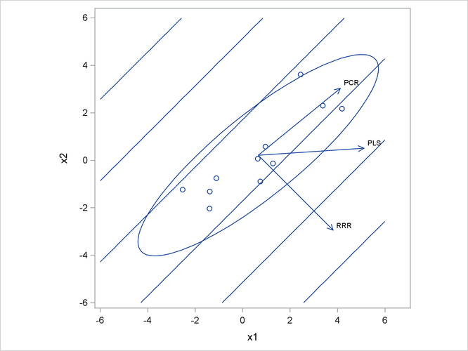
Figure 76.13: Depiction of First Factors for Three Different Regression Methods

The ellipse shows the general shape of the 11 observations in the predictor space, with the contours of increasing y overlaid. Also shown are the directions of the first factor for each of the three methods. Notice that, while the predictors vary most in the x1 = x2 direction, the response changes most in the orthogonal x1 = -x2 direction. This explains why the first principal component accounts for little variation in the response and why the first reduced rank regression factor accounts for little variation in the predictors. The direction of the first partial least squares factor represents a compromise between the other two directions.