The TPSPLINE Procedure
This example illustrates how you can construct a bootstrap confidence interval by using the multiple responses feature in PROC TPSPLINE.
Numerous epidemiological observations have indicated that exposure to solar radiation is an important factor in the etiology of melanoma. The following data present age-adjusted melanoma incidences for 37 years from the Connecticut Tumor Registry (Houghton, Flannery, and Viola, 1980). The data are analyzed by Ramsay and Silverman (1997).
data melanoma;
   input  year incidences @@;
   datalines;
1936    0.9   1937   0.8  1938   0.8  1939   1.3
1940    1.4   1941   1.2  1942   1.7  1943   1.8
1944    1.6   1945   1.5  1946   1.5  1947   2.0
1948    2.5   1949   2.7  1950   2.9  1951   2.5
1952    3.1   1953   2.4  1954   2.2  1955   2.9
1956    2.5   1957   2.6  1958   3.2  1959   3.8
1960    4.2   1961   3.9  1962   3.7  1963   3.3
1964    3.7   1965   3.9  1966   4.1  1967   3.8
1968    4.7   1969   4.4  1970   4.8  1971   4.8
1972    4.8
;
The variable incidences records the number of melanoma cases per ![]() people for the years 1936 to 1972. The following model fits the data and requests a 90% Bayesian confidence interval along
with the estimate:
people for the years 1936 to 1972. The following model fits the data and requests a 90% Bayesian confidence interval along
with the estimate:
ods graphics on;
proc tpspline data=melanoma plots(only)=(criterionplot fitplot(clm));
   model incidences = (year) /alpha = 0.1;
   output out = result pred uclm lclm;
run;
The output is displayed in Output 103.5.1
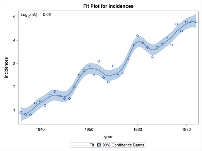
The estimated curve is displayed with 90% confidence interval bands in Output 103.5.2. The number of melanoma incidences exhibits a periodic pattern and increases over the years. The periodic pattern is related to sunspot activity and the accompanying fluctuations in solar radiation.
Wang and Wahba (1995) compare several bootstrap confidence intervals to Bayesian confidence intervals for smoothing splines. Both bootstrap and Bayesian confidence intervals are across-the-curve intervals, not pointwise intervals. They concluded that bootstrap confidence intervals work as well as Bayesian intervals concerning average coverage probability. Additionally, bootstrap confidence intervals appear to be better for small sample sizes. Based on their simulation, the "percentile-t interval" bootstrap interval performs better than the other types of bootstrap intervals.
Suppose that ![]() and
and ![]() are the estimates of f and
are the estimates of f and ![]() from the data. Assume that
from the data. Assume that ![]() is the "true" f, and generate the bootstrap sample as
is the "true" f, and generate the bootstrap sample as
where ![]() . Denote
. Denote ![]() as the random variable of the bootstrap estimate at
as the random variable of the bootstrap estimate at ![]() . Repeat this process K times, so that at each point
. Repeat this process K times, so that at each point ![]() , you have K bootstrap estimates
, you have K bootstrap estimates ![]() or K realizations of
or K realizations of ![]() . For each fixed
. For each fixed ![]() , consider the statistic
, consider the statistic ![]() , which is similar to the Student’s t statistic,
, which is similar to the Student’s t statistic,
where ![]() is the estimate of
is the estimate of ![]() based on the ith bootstrap sample.
based on the ith bootstrap sample.
Suppose ![]() and
and ![]() are the lower and upper
are the lower and upper ![]() points, respectively, of the empirical distribution of
points, respectively, of the empirical distribution of ![]() . The
. The ![]() 100% bootstrap confidence interval is defined as
100% bootstrap confidence interval is defined as
Bootstrap confidence intervals are easy to interpret and can be used with any distribution. However, because they require K model fits, their construction is computationally intensive.
The feature of multiple dependent variables in PROC TPSPLINE enables you to fit multiple models with the same independent variables. The procedure calculates the matrix decomposition part of the calculations only once, regardless of the number of dependent variables in the model. These calculations are responsible for most of the computing time used by the TPSPLINE procedure. This feature is particularly useful when you need to generate a bootstrap confidence interval.
To construct a bootstrap confidence interval, perform the following tasks:
-
Fit the data by using PROC TPSPLINE and obtain estimates
 and
and  .
.
-
Generate K bootstrap samples based on
 and
and  .
.
-
Fit the K bootstrap samples with the TPSPLINE procedure to obtain estimates of
 and
and  .
.
-
Compute
 and the values
  and
and  .
.
The following statements illustrate this process:
proc tpspline data=melanoma plots(only)=fitplot(clm);
   model incidences = (year) /alpha = 0.1;
   output out=result pred uclm lclm;
run;
The output from the initial PROC TPSPLINE analysis is displayed in Output 103.5.3. The data set result contains the predicted values and confidence limits from the analysis.
The following statements illustrate how you can obtain a bootstrap confidence interval for the Melanoma data set. The following statements create the data set bootstrap. The observations are created with information from the preceding PROC TPSPLINE execution; as displayed in Output 103.5.3, ![]() . The values of
. The values of ![]() are stored in the data set
are stored in the data set result in the variable P_incidence.
data bootstrap;
   set result;
   array y{1070} y1-y1070;
   do i=1 to 1070;
      y{i} = p_incidences + 0.232823*rannor(123456789);
   end;
   keep y1-y1070 p_incidences year;
run;

ods listing close;
proc tpspline data=bootstrap plots=none;
   ods output FitStatistics=FitResult;
   id p_incidences;
   model y1-y1070 = (year);
   output out=result2;
run;
ods listing;
The DATA step generates 1,070 bootstrap samples based on the previous estimate from PROC TPSPLINE. For this data set, some
of the bootstrap samples result in ![]() s (selected by the GCV function) that cause problematic behavior. Thus, an additional 70 bootstrap samples are generated.
s (selected by the GCV function) that cause problematic behavior. Thus, an additional 70 bootstrap samples are generated.
The ODS listing destination is closed before PROC TPSPLINE is invoked. The PLOTS=NONE option suppresses all graphical output.
The model fits all the y1…y1070 variables as dependent variables, and the models are fit for all bootstrap samples simultaneously. The output data set result2 contains the variables year, y1…y1070, p_y1…p_y1070, and p_incidences.
The ODS OUTPUT statement writes the FitStatistics table to the data set FitResult. The data set FitResult contains the two variables Parameter and Value. The FitResult data set is used in subsequent calculations for ![]() .
.
In the data set FitResult, there are 63 estimates with a standard deviation of zero, suggesting that the estimates provide perfect fits of the data
and are caused by ![]() s that are approximately equal to zero. For small sample sizes, there is a positive probability that the
s that are approximately equal to zero. For small sample sizes, there is a positive probability that the ![]() chosen by the GCV function will be zero (Wang and Wahba, 1995).
chosen by the GCV function will be zero (Wang and Wahba, 1995).
In the following steps, these cases are removed from the bootstrap samples as "bad" samples: they represent failure of the GCV function.
The following SAS statements manipulate the data set FitResult, retaining the standard deviations for all bootstrap samples and merging FitResult with the data set result2, which contains the estimates for bootstrap samples. In the final data set boot, the ![]() statistics are calculated.
statistics are calculated.
data FitResult;
   set FitResult;
   if Parameter="Standard Deviation";
   keep Value;
run;

proc transpose data=FitResult out=sd prefix=sd;

data result2;
   if _N_ = 1 then set sd;
   set result2;
run;

data boot;
   set result2;
   array y{1070}  p_y1-p_y1070;
   array sd{1070} sd1-sd1070;
   do i=1 to 1070;
      if sd{i} > 0 then do;
         d = (y{i} - P_incidences)/sd{i};
         obs = _N_;
         output;
      end;
   end;
   keep d obs P_incidences year;
run;
The following SAS statements retain the first 1,000 bootstrap samples and calculate the values ![]() and
and ![]() with
with ![]() .
.
proc sort data=boot;
   by obs;
run;

data boot;
   set boot;
      by obs;
   retain n;

   if first.obs then n=1;
      else n=n+1;
   if n > 1000 then delete;
run;

proc sort data=boot;
   by obs d;
run;

data chi1 chi2 ;
   set boot;
   if (_N_ = (obs-1)*1000+50)  then output chi1;
   if (_N_ = (obs-1)*1000+950) then output chi2;
run;

proc sort data=result;
   by year;
run;

proc sort data=chi1;
   by year;
run;

proc sort data=chi2;
   by year;
run;

data result;
   merge result
      chi1(rename=(d=chi05))
      chi2(rename=(d=chi95));
   keep year incidences P_incidences lower upper
        LCLM_incidences UCLM_incidences;

   lower = -chi95*0.232823 + P_incidences;
   upper = -chi05*0.232823 + P_incidences;

   label  lower="Lower 90% CL (Bootstrap)"
          upper="Upper 90% CL (Bootstrap)"
          lclm_incidences="Lower 90% CL (Bayesian)"
          uclm_incidences="Upper 90% CL (Bayesian)";
run;
The data set result contains the variables year and incidences, the PROC TPSPLINE estimate P_incidences, and the 90% Bayesian and 90% bootstrap confidence intervals.
The following statements produce Output 103.5.4:
proc sgplot data=result;
   title "Age-adjusted Melanoma Incidence for 37 Years";

   xaxis label="year";
   yaxis label="Incidences";

   band x=year lower=lclm_incidences upper=uclm_incidences/name="bayesian"
               legendlabel="90% Bayesian CI of Predicted incidences"
               fillattrs=(color=red);
   band x=year lower=lower upper=upper/name="bootstrap"
               legendlabel="90% Bootstrap CI of Predicted incidences"
               transparency=0.05;
   scatter x=year y=incidences/name="obs" legendlabel="incidences";
   series x=year y=p_incidences/name="pred"
               legendlabel="predicted values of incidences"
               lineattrs=graphfit(thickness=1px);

   discretelegend "bayesian" "bootstrap" "obs" "pred";
run;

ods graphics off;
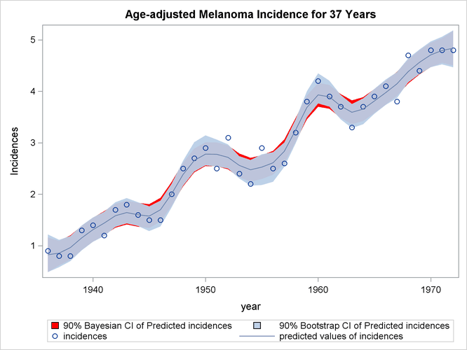
Output 103.5.4 displays the plot of the variable incidences, the predicted values, and the Bayesian and bootstrap confidence intervals.
The plot shows that the bootstrap confidence interval is similar to the Bayesian confidence interval. However, the Bayesian confidence interval is symmetric around the estimates, while the bootstrap confidence interval is not.


