The RELIABILITY Procedure
- Overview
-
Getting Started
 Analysis of Right-Censored Data from a Single PopulationWeibull Analysis Comparing Groups of DataAnalysis of Accelerated Life Test DataWeibull Analysis of Interval Data with Common Inspection ScheduleLognormal Analysis with Arbitrary CensoringRegression ModelingRegression Model with Nonconstant ScaleRegression Model with Two Independent VariablesWeibull Probability Plot for Two Combined Failure ModesAnalysis of Recurrence Data on RepairsComparison of Two Samples of Repair DataAnalysis of Interval Age Recurrence DataAnalysis of Binomial DataThree-Parameter WeibullParametric Model for Recurrent Events DataParametric Model for Interval Recurrent Events Data
 -
Syntax
 Primary StatementsSecondary StatementsGraphical Enhancement StatementsPROC RELIABILITY StatementANALYZE StatementBY StatementCLASS StatementDISTRIBUTION StatementEFFECTPLOT StatementESTIMATE StatementFMODE StatementFREQ StatementINSET StatementLOGSCALE StatementLSMEANS StatementLSMESTIMATE StatementMAKE StatementMCFPLOT StatementMODEL StatementNENTER StatementNLOPTIONS StatementPROBPLOT StatementRELATIONPLOT StatementSLICE StatementSTORE StatementTEST StatementUNITID Statement
 -
Details
 Abbreviations and NotationTypes of Lifetime DataProbability DistributionsProbability PlottingNonparametric Confidence Intervals for Cumulative Failure ProbabilitiesParameter Estimation and Confidence IntervalsRegression Model Statistics Computed for Each Observation for Lifetime DataRegression Model Statistics Computed for Each Observation for Recurrent Events DataRecurrence Data from Repairable SystemsODS Table NamesODS Graphics
 - References
Regression Model with Nonconstant Scale
Nelson (1990, p. 272) and Meeker and Escobar (1998, p. 439) analyzed data from a strain-controlled fatigue test on 26 specimens of a type of superalloy. The following SAS statements
create a SAS data set containing for each specimen the level of pseudo-stress (Pstress), the number of cycles (in thousands) (Kcycles) until failure or removal from the test, and a variable to indicate whether a specimen failed (F) or was right censored (C)
(Status):
data alloy;
   input pstress kCycles status$ @@;
   cen = ( status = 'C' );
   datalines;
80.3  211.629  F    99.8   43.331  F
80.6  200.027  F   100.1   12.076  F
80.8   57.923  C   100.5   13.181  F
84.3  155.000  F   113.0   18.067  F
85.2   13.949  F   114.8   21.300  F
85.6  112.968  C   116.4   15.616  F
85.8  152.680  F   118.0   13.030  F
86.4  156.725  F   118.4    8.489  F
86.7  138.114  C   118.6   12.434  F
87.2   56.723  F   120.4    9.750  F
87.3  121.075  F   142.5   11.865  F
89.7  122.372  C   144.5    6.705  F
91.3  112.002  F   145.9    5.733  F
;
The following statements fit a Weibull regression model with the number of cycles to failure as the response variable:
ods output ModObstats = Resids;
proc reliability data = alloy;
   distribution Weibull;
   model kcycles*cen(1) = pstress pstress*pstress / Relation = Pow Obstats;
   logscale pstress;
   rplot kcycles*cen(1) = pstress /  fit=regression
                                     relation = pow
                                     plotfit  10 50 90
                                     slower=60 supper=160
                                     lupper=500;

   label pstress = "Pseudo-Stress";
   label kcycles = "Thousands of Cycles";
run;
The data set RESIDS contains standardized residuals created with the ODS OUTPUT statement. The MODEL statement specifies a model quadratic in
the log of pseudo-stress for the extreme value location parameter. The quadratic model in pseudo-stress PSTRESS is specified
in the MODEL statement, and the RELATION=POW option specifies that the log transformation be applied to Pstress in the MODEL statement and the LOGSCALE statement. The LOGSCALE statement specifies the log of the scale parameter as a linear
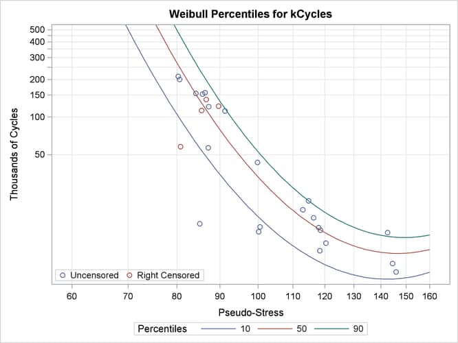
function of the log of Pstress. The RPLOT statement specifies a plot of the data and the fitted regression model versus the variable Pstress. The FIT=REGRESSION option specifies plotting the regression model fitted with the preceding MODEL statement. The RELATION=POW
option specifies a log stress axis. The PLOTFIT option specifies plotting the 10th, 50th, and 90th percentiles of the regression
model at each stress level. The SLOWER, SUPPER, and LUPPER options control limits on the stress and lifetime axes.
Figure 16.21 displays the parameter estimates from the fitted regression model. Parameter estimates for both the model for the location parameter and the scale parameter models are shown. Standard errors and confidence limits for all parameter estimates are included.
Figure 16.21: Parameter Estimates for Fitted Regression Model
| Weibull Parameter Estimates | ||||
|---|---|---|---|---|
| Parameter | Estimate | Standard Error | Asymptotic Normal | |
| 95% Confidence Limits | ||||
| Lower | Upper | |||
| Intercept | 243.1680 | 58.1777 | 129.1418 | 357.1943 |
| pstress | -96.5240 | 24.7558 | -145.0445 | -48.0035 |
| pstress*pstress | 9.6653 | 2.6299 | 4.5107 | 14.8198 |
| Log-Scale Parameter Estimates | ||||
|---|---|---|---|---|
| Parameter | Estimate | Standard Error | Asymptotic Normal | |
| 95% Confidence Limits | ||||
| Lower | Upper | |||
| Intercept | 4.4666 | 4.1745 | -3.7152 | 12.6484 |
| pstress | -1.1757 | 0.8950 | -2.9299 | 0.5784 |
Figure 16.22 displays the plot of the data and fitted regression model.
Figure 16.22: Superalloy Fatigue Data with Fitted Regression Model

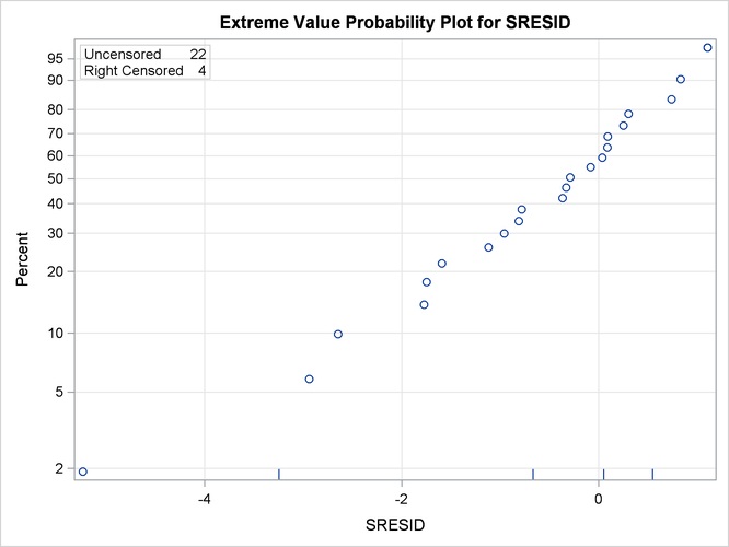
The following SAS statements create an extreme values probability plot of standardized residuals from the regression model shown in Figure 16.23:
proc reliability data = Resids;
   distribution ev;
   pplot sresid*cen(1) / nofit
                         ;
run;
Figure 16.23: Residuals for Superalloy Fatigue Data Regression Model
