Investigating Variability by Simulation :: SAS/STAT(R) 12.1 User's Guide

Investigating Variability by Simulation

The variability of $Z(\bm {s})$ , as modeled by

$Z(\bm {s}) = \mu + \varepsilon (\bm {s})$

with the Gaussian covariance structure $C_ z(\bm {h})$ found previously, is not obvious from the covariance model form and parameters. The variation around the mean of the surface is relatively small, making it difficult visually to pick up differences in surface plots of simulated realizations.

Instead, you can compute the mean for each location on a grid from a series of realizations in a simulation. Then, the standard deviation of all the simulated values at each grid location provides you with a measure of the variability of $Z(\bm {s})$ for the given covariance structure. You can also investigate variations at selected grid points in more detail, as shown in the Variability at Selected Locations.

The present example shows how to use ODS Graphics with PROC SIM2D to investigate the mean and standard deviation of simulated values. You use the thick data set which is available from the Sashelp library. In the data set, the Thick variable represents simulated observations of coal seam thickness. For your goal, you produce 5,000 realizations of a simulation with PROC SIM2D, where you specify the Gaussian model with the parameters found previously. You want the simulated data to pass through the simulated values, so first you define the data with the following data step:

title 'Using PROC SIM2D for Spatial Simulation';

data thick;
   input East North Thick @@;
   label Thick='Coal Seam Thickness';
   datalines;
    0.7  59.6  34.1   2.1  82.7  42.2   4.7  75.1  39.5
    4.8  52.8  34.3   5.9  67.1  37.0   6.0  35.7  35.9
    6.4  33.7  36.4   7.0  46.7  34.6   8.2  40.1  35.4
   13.3   0.6  44.7  13.3  68.2  37.8  13.4  31.3  37.8
   17.8   6.9  43.9  20.1  66.3  37.7  22.7  87.6  42.8
   23.0  93.9  43.6  24.3  73.0  39.3  24.8  15.1  42.3
   24.8  26.3  39.7  26.4  58.0  36.9  26.9  65.0  37.8
   27.7  83.3  41.8  27.9  90.8  43.3  29.1  47.9  36.7
   29.5  89.4  43.0  30.1   6.1  43.6  30.8  12.1  42.8
   32.7  40.2  37.5  34.8   8.1  43.3  35.3  32.0  38.8
   37.0  70.3  39.2  38.2  77.9  40.7  38.9  23.3  40.5
   39.4  82.5  41.4  43.0   4.7  43.3  43.7   7.6  43.1
   46.4  84.1  41.5  46.7  10.6  42.6  49.9  22.1  40.7
   51.0  88.8  42.0  52.8  68.9  39.3  52.9  32.7  39.2
   55.5  92.9  42.2  56.0   1.6  42.7  60.6  75.2  40.1
   62.1  26.6  40.1  63.0  12.7  41.8  69.0  75.6  40.1
   70.5  83.7  40.9  70.9  11.0  41.7  71.5  29.5  39.8
   78.1  45.5  38.7  78.2   9.1  41.7  78.4  20.0  40.8
   80.5  55.9  38.7  81.1  51.0  38.6  83.8   7.9  41.6
   84.5  11.0  41.5  85.2  67.3  39.4  85.5  73.0  39.8
   86.7  70.4  39.6  87.2  55.7  38.8  88.1   0.0  41.6
   88.4  12.1  41.3  88.4  99.6  41.2  88.8  82.9  40.5
   88.9   6.2  41.5  90.6   7.0  41.5  90.7  49.6  38.9
   91.5  55.4  39.0  92.9  46.8  39.1  93.4  70.9  39.7
   55.8  50.5  38.1  96.2  84.3  40.3  98.2  58.2  39.5
   ;

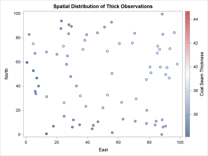
Since this is a conditional simulation, you can specify the OBSERV option in the PLOTS option in PROC SIM2D to see the locations and values of the measured points in the area where you want to perform spatial simulations.

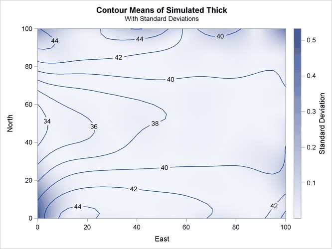
Furthermore, the SIM suboption in the PLOTS option specifies that you want to create a plot that shows the means of the simulated values across the region. The SIM suboption with no other arguments produces a plot that shows the contours of the simulated means in the foreground and the gradient of the simulated standard deviations in the background.

You obtain these PROC SIM2D results at the nodes of an output grid that you specify according to your application needs. In the present analysis, a convenient area that encompasses all the Thick data points is a square with a side length of 100,000 feet. You define a regular grid for your simulation in this area. Assume a distance of 2,500 feet between grid nodes in both directions for a smooth contour plot. Based on this choice, your square grid has 41 nodes on each side. This means that PROC SIM2D computes the simulated values at a total of 1,681 grid points. You use the GRID statement of the PROC SIM2D to specify this grid.

The SIMULATE statement specifies the parameters of your simulation across the output grid. In particular, the VAR= option specifies the conditional simulation variable. The number of realizations in the simulation is specified with the NUMREAL= option. The SEED= option specifies the seed for the simulation random number generator.

The spatial correlation model for the simulation is also specified in the SIMULATE statement. You specify the model type by using the FORM= option. The options SCALE= and RANGE= specify the covariance structure sill and range parameters, respectively, as discussed in the previous section.

Although it is not included in the original spatial structure, note that a minimal nugget effect is specified with the NUGGET= option to avoid singularity issues. Singularity can appear in the present example as a result of the combined use of the Gaussian covariance model and relatively short distances between nodes, data, or nodes and data in the simulation area.

These steps are implemented using the following DATA step and statements:

ods graphics on;

proc sim2d data=thick outsim=sim plot=(observ sim);
   coordinates xc=East yc=North;
   simulate var=Thick numreal=5000 seed=79931
      scale=7.4599 range=30.1111 nugget=1e-8 form=gauss;
   mean 40.1173;
   grid x=0 to 100 by 2.5 y=0 to 100 by 2.5;
run;

The table in Figure 85.1 shows the number of observations read and used in the conditional simulation. This table can provide you with useful information in case you have missing values in the input data.

Figure 85.1: Number of Observations for the thick Data Set

Using PROC SIM2D for Spatial Simulation

The SIM2D Procedure

Simulation: SIM1, Dependent Variable: Thick

Number of Observations Read	75
Number of Observations Used	75

The sample locations are then plotted in Figure 85.2. The figure clearly shows some small-scale variation that is typical of spatial data.

Figure 85.2: Scatter Plot of the Observations Spatial Distribution

PROC SIM2D also produces the table shown in Figure 85.3, which contains information about the type of simulation you run and the number of realizations requested.

Figure 85.3: Simulation Analysis Information

Simulation Information
Simulation Grid Points	1681
Type	Conditional
Number of Realizations	5000

The table in Figure 85.4 displays the spatial correlation model information that is used by PROC SIM2D for the current simulation. If applicable, the table also provides the effective range. This is the distance $r_{\epsilon }$ at which the covariance is 5% of its value at zero. Here you specified the Gaussian model, for which the effective range $r_{\epsilon }$ is $\sqrt {3}a_0$ .

Figure 85.4: Simulation Covariance Model Information

Covariance Model Information
Type	Gaussian
Sill	7.4599
Range	30.1111
Effective Range	52.153955
Nugget Effect	1E-8

Eventually, the SIM2D procedure produces the requested simulation plot shown in Figure 85.5. The contours of the mean of the simulated values show the average of the simulated realizations at each grid node; the average is based on the given spatial structure characteristics. In this case, these means are also conditioned by the Thick observations across the region.

Figure 85.5: Contour Plot of Conditionally Simulated Coal Seam Thickness

Observe also the gradient that shows the standard deviation of the simulated values at each grid node. This gradient appears to be generally small throughout the region. A few exceptions are evident close to the region borders. In these areas the simulated realizations depend on a limited amount of neighboring data. The simulation at these locations relies mainly on the underlying spatial structure.

In addition to the simulation analysis, you can use the PROC SIM2D output to obtain statistical information about the simulated values at selected locations. Assume that you would like some basic statistics for the extreme southwest point at (East=0, North=0) and the point (East=75, North=75) toward the northeast corner of the region. You use the following DATA step to select the realizations for these points from the OUTSIM= output data set:

data selected;
   set sim(where=((gxc=0 and gyc=0) or (gxc=75 and gyc=75)));
   label gxc = "X-coord";
   label gyc = "Y-coord";
run;

Then, you use PROC SORT to sort the selected data set entries and PROC MEANS to produce the simulation statistics for the selected points. The following statements yield the mean, standard deviation, and maximum values of the 5,000 realizations of the Thick values at each one of the selected locations:

proc sort data=selected;
   by gxc gyc;
run;
proc means data=selected Mean Std Max;
   class gxc gyc;
   ways 2;
   where (  ((gxc =  0) & (gyc =  0))
          | ((gxc = 75) & (gyc = 75)));
   var SValue;
run;

ods graphics off;

The requested statistics for the grid points (East=0, North=0) and (East=75,North=75) are shown in Figure 85.6.

Figure 85.6: Simulation Statistics at Grid Points (East=0, North=0) and (East=75, North=75)

Using PROC SIM2D for Spatial Simulation

The MEANS Procedure

Analysis Variable : SVALUE Simulated Value at Grid Point
X-coord	Y-coord	N Obs	Mean	Std Dev	Maximum
0	0	5000	40.6968472	0.5328597	42.6616357
75	75	5000	40.1090845	0.0024556	40.1197239

Variability at Selected Locations shows you how to perform a simulation at a set of selected locations rather than on a domain-wide grid, and how to obtain more detailed statistics from the simulation.