The REG Procedure
- Overview
-
Getting Started

-
Syntax

-
Details
 Missing ValuesInput Data SetsOutput Data SetsInteractive AnalysisModel-Selection MethodsCriteria Used in Model-Selection MethodsLimitations in Model-Selection MethodsParameter Estimates and Associated StatisticsPredicted and Residual ValuesModels of Less Than Full RankCollinearity DiagnosticsModel Fit and Diagnostic StatisticsInfluence StatisticsReweighting Observations in an AnalysisTesting for HeteroscedasticityTesting for Lack of FitMultivariate TestsAutocorrelation in Time Series DataComputations for Ridge Regression and IPC AnalysisConstruction of Q-Q and P-P PlotsComputational MethodsComputer Resources in Regression AnalysisDisplayed OutputPlot Options Superseded by ODS GraphicsODS Table NamesODS Graphics
 -
Examples

- References
This example uses the acetylene data in Marquardt and Snee (1975) to illustrate the RIDGEPLOT and OUTVIF options. Here are the data:
data acetyl;
   input x1-x4 @@;
   x1x2 = x1 * x2;
   x1x1 = x1 * x1;
   label x1  = 'reactor temperature(celsius)'
         x2  = 'h2 to n-heptone ratio'
         x3  = 'contact time(sec)'
         x4  = 'conversion percentage'
         x1x2= 'temperature-ratio interaction'
         x1x1= 'squared temperature';
   datalines;
1300  7.5 .012 49   1300  9   .012  50.2 1300 11 .0115 50.5
1300 13.5 .013 48.5 1300 17   .0135 47.5 1300 23 .012  44.5
1200  5.3 .04  28   1200  7.5 .038  31.5 1200 11 .032  34.5
1200 13.5 .026 35   1200 17   .034  38   1200 23 .041  38.5
1100  5.3 .084 15   1100  7.5 .098  17   1100 11 .092  20.5
1100 17   .086 29.5
;
ods graphics on;

proc reg data=acetyl outvif
         outest=b ridge=0 to 0.02 by .002;
   model x4=x1 x2 x3 x1x2 x1x1;
run;
proc print data=b;
run;
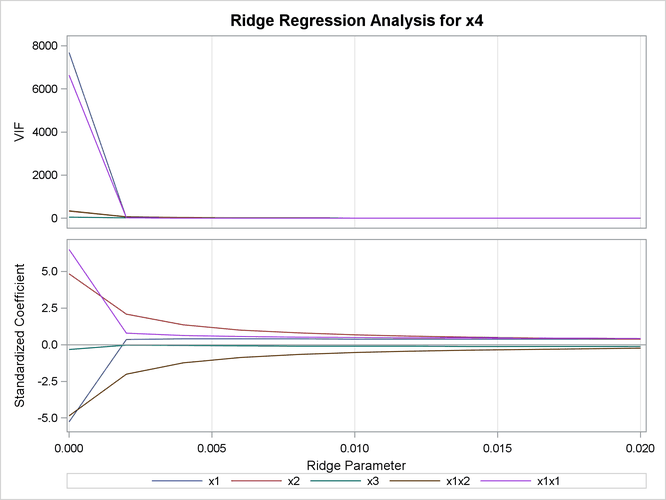
When ODS Graphics is enabled and you request ridge regression by using the RIDGE= option in the PROC REG statement, PROC REG produces a panel showing variance inflation factors (VIF) in the upper plot in the panel and ridge traces in the lower plot. This panel is shown in Output 85.5.1.
The OUTVIF option outputs the variance inflation factors to the OUTEST= data set that is shown in Output 85.5.2.
Output 85.5.2: OUTEST Data Set Showing VIF Values
| Obs | _MODEL_ | _TYPE_ | _DEPVAR_ | _RIDGE_ | _PCOMIT_ | _RMSE_ | Intercept | x1 | x2 | x3 | x1x2 | x1x1 | x4 |
|---|---|---|---|---|---|---|---|---|---|---|---|---|---|
| 1 | MODEL1 | PARMS | x4 | . | . | 1.15596 | 390.538 | -0.78 | 10.174 | -121.626 | -0.008 | 0.00 | -1 |
| 2 | MODEL1 | RIDGEVIF | x4 | 0.000 | . | . | . | 7682.37 | 320.022 | 53.525 | 344.545 | 6643.32 | -1 |
| 3 | MODEL1 | RIDGE | x4 | 0.000 | . | 1.15596 | 390.538 | -0.78 | 10.174 | -121.626 | -0.008 | 0.00 | -1 |
| 4 | MODEL1 | RIDGEVIF | x4 | 0.002 | . | . | . | 11.18 | 58.731 | 10.744 | 63.208 | 11.22 | -1 |
| 5 | MODEL1 | RIDGE | x4 | 0.002 | . | 2.69721 | -103.388 | 0.05 | 4.404 | -9.065 | -0.003 | 0.00 | -1 |
| 6 | MODEL1 | RIDGEVIF | x4 | 0.004 | . | . | . | 4.36 | 23.939 | 9.996 | 25.744 | 5.15 | -1 |
| 7 | MODEL1 | RIDGE | x4 | 0.004 | . | 3.22340 | -93.797 | 0.06 | 2.839 | -21.338 | -0.002 | 0.00 | -1 |
| 8 | MODEL1 | RIDGEVIF | x4 | 0.006 | . | . | . | 2.93 | 13.011 | 9.383 | 13.976 | 3.81 | -1 |
| 9 | MODEL1 | RIDGE | x4 | 0.006 | . | 3.47752 | -87.687 | 0.06 | 2.110 | -28.447 | -0.001 | 0.00 | -1 |
| 10 | MODEL1 | RIDGEVIF | x4 | 0.008 | . | . | . | 2.36 | 8.224 | 8.838 | 8.821 | 3.23 | -1 |
| 11 | MODEL1 | RIDGE | x4 | 0.008 | . | 3.62677 | -83.593 | 0.06 | 1.689 | -33.377 | -0.001 | 0.00 | -1 |
| 12 | MODEL1 | RIDGEVIF | x4 | 0.010 | . | . | . | 2.04 | 5.709 | 8.343 | 6.112 | 2.89 | -1 |
| 13 | MODEL1 | RIDGE | x4 | 0.010 | . | 3.72505 | -80.603 | 0.06 | 1.414 | -37.177 | -0.001 | 0.00 | -1 |
| 14 | MODEL1 | RIDGEVIF | x4 | 0.012 | . | . | . | 1.84 | 4.226 | 7.891 | 4.514 | 2.65 | -1 |
| 15 | MODEL1 | RIDGE | x4 | 0.012 | . | 3.79477 | -78.276 | 0.06 | 1.221 | -40.297 | -0.001 | 0.00 | -1 |
| 16 | MODEL1 | RIDGEVIF | x4 | 0.014 | . | . | . | 1.69 | 3.279 | 7.476 | 3.493 | 2.46 | -1 |
| 17 | MODEL1 | RIDGE | x4 | 0.014 | . | 3.84693 | -76.381 | 0.06 | 1.078 | -42.965 | -0.001 | 0.00 | -1 |
| 18 | MODEL1 | RIDGEVIF | x4 | 0.016 | . | . | . | 1.57 | 2.637 | 7.094 | 2.801 | 2.31 | -1 |
| 19 | MODEL1 | RIDGE | x4 | 0.016 | . | 3.88750 | -74.785 | 0.06 | 0.968 | -45.309 | -0.001 | 0.00 | -1 |
| 20 | MODEL1 | RIDGEVIF | x4 | 0.018 | . | . | . | 1.47 | 2.182 | 6.741 | 2.310 | 2.18 | -1 |
| 21 | MODEL1 | RIDGE | x4 | 0.018 | . | 3.92004 | -73.407 | 0.06 | 0.880 | -47.407 | -0.000 | 0.00 | -1 |
| 22 | MODEL1 | RIDGEVIF | x4 | 0.020 | . | . | . | 1.39 | 1.847 | 6.415 | 1.949 | 2.06 | -1 |
| 23 | MODEL1 | RIDGE | x4 | 0.020 | . | 3.94679 | -72.193 | 0.06 | 0.809 | -49.310 | -0.000 | 0.00 | -1 |
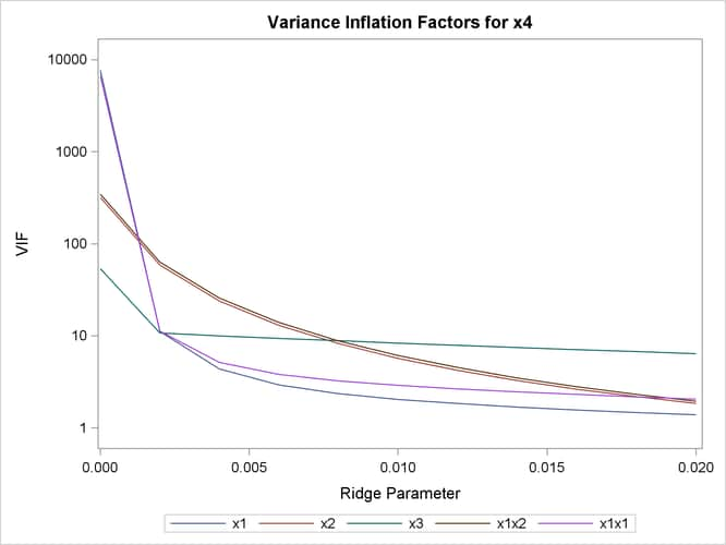
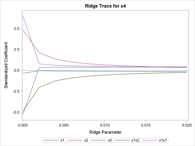
If you want to obtain separate plots containing the ridge traces and VIF traces, you can specify the UNPACK suboption in the PLOTS=RIDGE option. You can also request that one or both of the VIF axis and ridge parameter axis be displayed on a logarithmic scale. You can see in Output 85.5.1 that the VIF traces for several of the parameters are nearly indistinguishable when displayed on a linear scale. The following code illustrates how you obtain separate VIF and ridge traces with the VIF values displayed on a logarithmic scale. Note that you can obtain plots of VIF values even though you do not specify the OUTVIF option in the PROC REG statement.
proc reg data=acetyl plots(only)=ridge(unpack VIFaxis=log)
         outest=b ridge=0 to 0.02 by .002;
   model x4=x1 x2 x3 x1x2 x1x1;
run;

ods graphics off;
The requested plots are shown in Output 85.5.3 and Output 85.5.4.


