The UNIVARIATE Procedure

Calculating Percentiles

Subsections:

Weighted Percentiles
Confidence Limits for Percentiles

The UNIVARIATE procedure automatically computes the 1st, 5th, 10th, 25th, 50th, 75th, 90th, 95th, and 99th percentiles (quantiles), as well as the minimum and maximum of each analysis variable. To compute percentiles other than these default percentiles, use the PCTLPTS= and PCTLPRE= options in the OUTPUT statement.

You can specify one of five definitions for computing the percentiles with the PCTLDEF= option. Let $n$ be the number of nonmissing values for a variable, and let $x_1, x_2, \ldots , x_ n$ represent the ordered values of the variable. Let the $t$ th percentile be $y$ , set $p = \frac{t}{100}$ , and let

$\begin{array}{rcll} np & =& j+g & ~ ~ \mbox{when PCTLDEF=1, 2, 3, or 5} \\ (n + 1) p & =& j+g & ~ ~ \mbox{when PCTLDEF=4} \end{array}$

where $j$ is the integer part of np, and $g$ is the fractional part of np. Then the PCTLDEF= option defines the $t$ th percentile, $y$ , as described in the following table.

PCTLDEF	Description	Formula
1	weighted average at $x_{np}$	$y = (1-g)x_ j+gx_{j+1}$
		where $x_{0}$ is taken to be $x_{1}$
2	observation numbered closest to np	$\begin{array}{ll} y=x_ j & \mbox{if } g < \frac{1}{2} \\ y=x_ j & \mbox{if } g=\frac{1}{2} \mbox{ and } \mi {j} \mbox{ is even} \\ y=x_{j+1} & \mbox{if } g=\frac{1}{2} \mbox{ and } \mi {j} \mbox{ is odd} \\ y=x_{j+1} & \mbox{if } g > \frac{1}{2} \\ \end{array}$
3	empirical distribution function	$\begin{array}{ll} y=x_{j} & \mbox{if } g=0 \\ y=x_{j+1} & \mbox{if } g>0 \end{array}$
4	weighted average aimed	$y=(1-g)x_ j + gx_{j+1}$
	at $x_{(n + 1) p}$	where $x_{n + 1}$ is taken to be $x_ n$
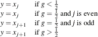
5	empirical distribution function with averaging	$\begin{array}{ll} y=\frac{1}{2}(x_ j + x_{j+1}) & \mbox{if } g=0 \\ y=x_{j+1} & \mbox{if } g>0 \end{array}$

Weighted Percentiles

When you use a WEIGHT statement, the percentiles are computed differently. The 100 $p$ th weighted percentile $y$ is computed from the empirical distribution function with averaging:

$y = \left\{ \begin{array}{cl} x_1 & \mbox{if} \ w_1 > pW \\ \frac{1}{2} ( x_ i + x_{i+1} ) & \mbox{if} \sum _{j=1}^{i} w_ j = pW \\ x_{i+1} & \mbox{if} \sum _{j=1}^{i} w_ j < pW < \sum _{j=1}^{i+1} w_ j \end{array} \right.$

where $w_ i$ is the weight associated with $x_ i$ and $W = \sum _{i=1}^{n} w_ i$ is the sum of the weights.

Note that the PCTLDEF= option is not applicable when a WEIGHT statement is used. However, in this case, if all the weights are identical, the weighted percentiles are the same as the percentiles that would be computed without a WEIGHT statement and with PCTLDEF=5.

Confidence Limits for Percentiles

You can use the CIPCTLNORMAL option to request confidence limits for percentiles, assuming the data are normally distributed. These limits are described in Section 4.4.1 of Hahn and Meeker (1991). When $0 < p < \frac{1}{2}$ , the two-sided $100(1-\alpha )\%$ confidence limits for the $100p$ th percentile are

$\begin{array}{lcl} \mbox{lower limit} & = & \bar{X} - g’(\frac{\alpha }{2};1-p,n) s \\ \mbox{upper limit} & = & \bar{X} - g’(1 - \frac{\alpha }{2};p,n) s \end{array}$

where $n$ is the sample size. When $\frac{1}{2} \leq p < 1$ , the two-sided $100(1-\alpha )\%$ confidence limits for the $100p$ th percentile are

$\begin{array}{lcl} \mbox{lower limit} & = & \bar{X} + g’(\frac{\alpha }{2};1-p,n) s \\ \mbox{upper limit} & = & \bar{X} + g’(1 - \frac{\alpha }{2};p,n) s \end{array}$

One-sided $100(1-\alpha )\%$ confidence bounds are computed by replacing $\frac{\alpha }{2}$ by $\alpha$ in the appropriate preceding equation. The factor $g’(\gamma ,p,n)$ is related to the noncentral $t$ distribution and is described in Owen and Hua (1977) and Odeh and Owen (1980). See Example 4.10.

You can use the CIPCTLDF option to request distribution-free confidence limits for percentiles. In particular, it is not necessary to assume that the data are normally distributed. These limits are described in Section 5.2 of Hahn and Meeker (1991). The two-sided $100(1-\alpha )\%$ confidence limits for the $100p$ th percentile are

$\begin{array}{lcl} \mbox{lower limit} & = & X_{(l)} \\ \mbox{upper limit} & = & X_{(u)} \end{array}$

where $X_{(j)}$ is the $j$ th order statistic when the data values are arranged in increasing order:

$X_{(1)} \leq X_{(2)} \leq \ldots \leq X_{(n)}$

The lower rank $l$ and upper rank $u$ are integers that are symmetric (or nearly symmetric) around $\lfloor np \rfloor +1$ , where $\lfloor np \rfloor$ is the integer part of $np$ and $n$ is the sample size. Furthermore, $l$ and $u$ are chosen so that $X_{(l)}$ and $X_{(u)}$ are as close to $X_{\lfloor np \rfloor +1}$ as possible while satisfying the coverage probability requirement,

$Q(u-1;n,p) - Q(l-1;n,p) \geq 1 - \alpha$

where $Q(k;n,p)$ is the cumulative binomial probability,

$Q(k;n,p) = \sum _{i=0}^{k} \left(\begin{array}{c} n \cr i \end{array}\right) p^ i (1-p)^{n-i}$

In some cases, the coverage requirement cannot be met, particularly when $n$ is small and $p$ is near 0 or 1. To relax the requirement of symmetry, you can specify CIPCTLDF(TYPE = ASYMMETRIC). This option requests symmetric limits when the coverage requirement can be met, and asymmetric limits otherwise.

If you specify CIPCTLDF(TYPE = LOWER), a one-sided $100(1-\alpha )\%$ lower confidence bound is computed as $X_{(l)}$ , where $l$ is the largest integer that satisfies the inequality

$1 - Q(l-1;n,p) \geq 1 - \alpha$

with $0 < l \leq n$ . Likewise, if you specify CIPCTLDF(TYPE = UPPER), a one-sided $100(1-\alpha )\%$ lower confidence bound is computed as $X_{(u)}$ , where $u$ is the largest integer that satisfies the inequality

$Q(u-1;n,p) \geq 1 - \alpha \; \; \; \mbox{ where } 0 < u \leq n$

Note that confidence limits for percentiles are not computed when a WEIGHT statement is specified. See Example 4.10.