The UNIVARIATE Procedure
- Overview
-
Getting Started

-
Syntax

-
Details
 Missing ValuesRoundingDescriptive StatisticsCalculating the ModeCalculating PercentilesTests for LocationConfidence Limits for Parameters of the Normal DistributionRobust EstimatorsCreating Line Printer PlotsCreating High-Resolution GraphicsUsing the CLASS Statement to Create Comparative PlotsPositioning InsetsFormulas for Fitted Continuous DistributionsGoodness-of-Fit TestsKernel Density EstimatesConstruction of Quantile-Quantile and Probability PlotsInterpretation of Quantile-Quantile and Probability PlotsDistributions for Probability and Q-Q PlotsEstimating Shape Parameters Using Q-Q PlotsEstimating Location and Scale Parameters Using Q-Q PlotsEstimating Percentiles Using Q-Q PlotsInput Data SetsOUT= Output Data Set in the OUTPUT StatementOUTHISTOGRAM= Output Data SetOUTKERNEL= Output Data SetOUTTABLE= Output Data SetTables for Summary StatisticsODS Table NamesODS Tables for Fitted DistributionsODS GraphicsComputational Resources
 -
Examples
 Computing Descriptive Statistics for Multiple VariablesCalculating ModesIdentifying Extreme Observations and Extreme ValuesCreating a Frequency TableCreating Plots for Line Printer OutputAnalyzing a Data Set With a FREQ VariableSaving Summary Statistics in an OUT= Output Data SetSaving Percentiles in an Output Data SetComputing Confidence Limits for the Mean, Standard Deviation, and VarianceComputing Confidence Limits for Quantiles and PercentilesComputing Robust EstimatesTesting for LocationPerforming a Sign Test Using Paired DataCreating a HistogramCreating a One-Way Comparative HistogramCreating a Two-Way Comparative HistogramAdding Insets with Descriptive StatisticsBinning a HistogramAdding a Normal Curve to a HistogramAdding Fitted Normal Curves to a Comparative HistogramFitting a Beta CurveFitting Lognormal, Weibull, and Gamma CurvesComputing Kernel Density EstimatesFitting a Three-Parameter Lognormal CurveAnnotating a Folded Normal CurveCreating Lognormal Probability PlotsCreating a Histogram to Display Lognormal FitCreating a Normal Quantile PlotAdding a Distribution Reference LineInterpreting a Normal Quantile PlotEstimating Three Parameters from Lognormal Quantile PlotsEstimating Percentiles from Lognormal Quantile PlotsEstimating Parameters from Lognormal Quantile PlotsComparing Weibull Quantile PlotsCreating a Cumulative Distribution PlotCreating a P-P Plot
 - References
You can use the CDFPLOT, HISTOGRAM, PPPLOT, PROBPLOT, and QQPLOT statements to create high-resolution graphs.
The CDFPLOT statement plots the observed cumulative distribution function of a variable. You can optionally superimpose a fitted theoretical distribution on the plot.
The HISTOGRAM statement creates histograms that enable you to examine the data distribution. You can optionally fit families of density curves and superimpose kernel density estimates on the histograms. For additional information about the fitted distributions and kernel density estimates, see the sections Formulas for Fitted Continuous Distributions and Kernel Density Estimates.
The PPPLOT statement creates a probability-probability (P-P) plot, which compares the empirical cumulative distribution function (ECDF) of a variable with a specified theoretical cumulative distribution function. You can use a P-P plot to determine how well a theoretical distribution models a set of measurements.
The PROBPLOT statement creates a probability plot, which compares ordered values of a variable with percentiles of a specified theoretical distribution. Probability plots are useful for graphical estimation of percentiles.
The QQPLOT statement creates a quantile-quantile plot, which compares ordered values of a variable with quantiles of a specified theoretical distribution. Q-Q plots are useful for graphical estimation of distribution parameters.
Note: You can use the CLASS statement with any of these plot statements to produce comparative versions of the plots.
The UNIVARIATE procedure supports two kinds of graphical output.
-
ODS Statistical Graphics output is produced if ODS Graphics is enabled, for example by specifying the ODS GRAPHICS ON statement prior to the PROC statement.
-
Otherwise, traditional graphics are produced if SAS/GRAPH® is licensed.
Traditional graphics are saved in graphics catalogs. Their appearance is controlled by the SAS/GRAPH GOPTIONS, AXIS, and SYMBOL statements (as described in SAS/GRAPH: Reference) and numerous specialized plot statement options.
ODS Statistical Graphics (or ODS Graphics for short) is an extension to the Output Delivery System (ODS) that can be enabled by specifying the ODS GRAPHICS statement prior to your procedure statements. An ODS graph is produced in ODS output (not a graphics catalog), and the details of its appearance and layout are controlled by ODS styles and templates rather than by SAS/GRAPH statements and procedure options. See Chapter 21: Statistical Graphics Using ODS in SAS/STAT User's Guide, for a thorough discussion of ODS Graphics.
Prior to SAS 9.2, the plots produced by PROC UNIVARIATE were extremely basic by default. Producing attractive graphical output required the careful selection of colors, fonts, and other elements, which were specified via SAS/GRAPH statements and plot statement options. Beginning with SAS 9.2, the default appearance of traditional graphs is governed by the prevailing ODS style, which automatically produces attractive, consistent output. The SAS/GRAPH statements and procedure options for controlling graph appearance continue to be honored for traditional graphics. You can specify the NOGSTYLE system option to prevent the ODS style from affecting the appearance of traditional graphs. This enables existing PROC UNIVARIATE programs to produce customized graphs that appear as they did under previous SAS releases.
The appearance of ODS Graphics output is also controlled by the ODS style, but it is not affected by SAS/GRAPH statements or plot statement options that govern traditional graphics, For example, the CAXIS= option used to specify the color of graph axes in traditional graphics is ignored when producing ODS Graphics output. Note: Some features available with traditional graphics are not supported in ODS Graphics by the UNIVARIATE procedure for SAS 9.2.
The traditional graphics system enables you to control every detail of a graph through convenient procedure syntax. ODS Graphics provides the highest quality output with minimal syntax and full compatibility with graphics produced by SAS/STAT and SAS/ETS procedures.
The following code produces a histogram with a fitted lognormal distribution of the LoanToValueRatio data introduced in the section Summarizing a Data Distribution:
options nogstyle;
ods graphics off;
proc univariate data=HomeLoans noprint;
   histogram LoanToValueRatio / lognormal;
   inset lognormal(theta sigma zeta) / position=ne;
run;
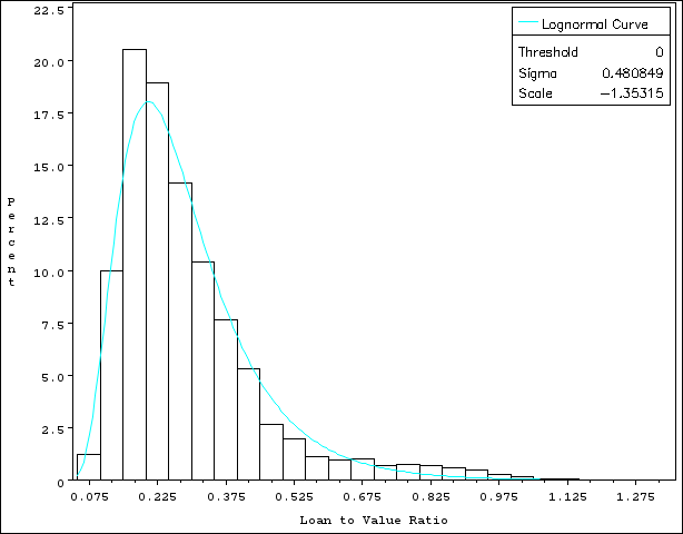
The NOGSTYLE system option keeps the ODS style from influencing the output, and no SAS/GRAPH statements or procedure options affecting the appearance of the plot are specified. Figure 4.8 shows the resulting histogram, which is essentially identical to the default output produced under releases prior to SAS 9.2.
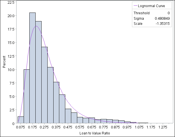
Figure 4.9 shows the result of executing the same code with the GSTYLE system option turned on (the default). Note the influence of the ODS style on the histogram’s appearance. For example, the quality of the text is improved and histogram bars are filled by default.
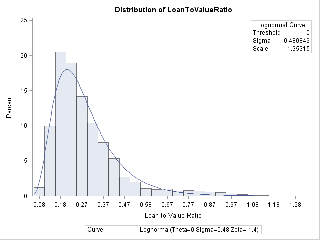
Figure 4.10 shows the same histogram produced using ODS Graphics. The histogram’s appearance is governed by the same style elements as in Figure 4.9, but the plots are not identical. Note, for example, the title incorporated in the ODS Graphics output and the smoother appearance of the fitted curve.


