The GLIMMIX Procedure
-
Overview

-
Getting Started
-
SyntaxPROC GLIMMIX StatementBY StatementCLASS StatementCODE StatementCONTRAST StatementCOVTEST StatementEFFECT StatementESTIMATE StatementFREQ StatementID StatementLSMEANS StatementLSMESTIMATE StatementMODEL StatementNLOPTIONS StatementOUTPUT StatementPARMS StatementRANDOM StatementSLICE StatementSTORE StatementWEIGHT StatementProgramming StatementsUser-Defined Link or Variance Function
-
DetailsGeneralized Linear Models TheoryGeneralized Linear Mixed Models TheoryGLM Mode or GLMM ModeStatistical Inference for Covariance ParametersDegrees of Freedom MethodsEmpirical Covariance (Sandwich) EstimatorsExploring and Comparing Covariance MatricesProcessing by SubjectsRadial Smoothing Based on Mixed ModelsOdds and Odds Ratio EstimationParameterization of Generalized Linear Mixed ModelsResponse-Level Ordering and ReferencingComparing the GLIMMIX and MIXED ProceduresSingly or Doubly Iterative FittingDefault Estimation TechniquesDefault OutputNotes on Output StatisticsODS Table NamesODS Graphics
-
ExamplesBinomial Counts in Randomized BlocksMating Experiment with Crossed Random EffectsSmoothing Disease Rates; Standardized Mortality RatiosQuasi-likelihood Estimation for Proportions with Unknown DistributionJoint Modeling of Binary and Count DataRadial Smoothing of Repeated Measures DataIsotonic Contrasts for Ordered AlternativesAdjusted Covariance Matrices of Fixed EffectsTesting Equality of Covariance and Correlation MatricesMultiple Trends Correspond to Multiple Extrema in Profile LikelihoodsMaximum Likelihood in Proportional Odds Model with Random EffectsFitting a Marginal (GEE-Type) ModelResponse Surface Comparisons with Multiplicity AdjustmentsGeneralized Poisson Mixed Model for Overdispersed Count DataComparing Multiple B-SplinesDiallel Experiment with Multimember Random EffectsLinear Inference Based on Summary Data
- References
Confidence Bounds Based on Likelihoods
Families of statistical tests can be inverted to produce confidence limits for parameters. The confidence region for parameter
![]() is the set of values for which the corresponding test fails to reject
is the set of values for which the corresponding test fails to reject ![]() . When parameters are estimated by maximum likelihood or a likelihood-based technique, it is natural to consider the likelihood
ratio test statistic for H in the test inversion. When there are multiple parameters in the model, however, you need to supply values for these nuisance
parameters during the test inversion as well.
. When parameters are estimated by maximum likelihood or a likelihood-based technique, it is natural to consider the likelihood
ratio test statistic for H in the test inversion. When there are multiple parameters in the model, however, you need to supply values for these nuisance
parameters during the test inversion as well.
In the following, suppose that ![]() is the covariance parameter vector and that one of its elements,
is the covariance parameter vector and that one of its elements, ![]() , is the parameter of interest for which you want to construct a confidence interval. The other elements of
, is the parameter of interest for which you want to construct a confidence interval. The other elements of ![]() are collected in the nuisance parameter vector
are collected in the nuisance parameter vector ![]() . Suppose that
. Suppose that ![]() is the estimate of
is the estimate of ![]() from the overall optimization and that
from the overall optimization and that ![]() is the likelihood evaluated at that estimate. If estimation is based on pseudo-data, then
is the likelihood evaluated at that estimate. If estimation is based on pseudo-data, then ![]() is the pseudo-likelihood based on the final pseudo-data. If estimation uses a residual (restricted) likelihood, then L denotes the restricted maximum likelihood and
is the pseudo-likelihood based on the final pseudo-data. If estimation uses a residual (restricted) likelihood, then L denotes the restricted maximum likelihood and ![]() is the REML estimate.
is the REML estimate.
Profile Likelihood Bounds
The likelihood ratio test statistic for testing ![]() is
is
|
|
where ![]() is the likelihood estimate of
is the likelihood estimate of ![]() under the restriction that
under the restriction that ![]() . To invert this test, a function is defined that returns the maximum likelihood for a fixed value of
. To invert this test, a function is defined that returns the maximum likelihood for a fixed value of ![]() by seeking the maximum over the remaining parameters. This function is termed the profile likelihood (Pawitan, 2001, Ch. 3.4),
by seeking the maximum over the remaining parameters. This function is termed the profile likelihood (Pawitan, 2001, Ch. 3.4),
|
|
In computing ![]() ,
, ![]() is fixed at
is fixed at ![]() and
and ![]() is estimated. In mixed models, this step typically requires a separate, iterative optimization to find the estimate of
is estimated. In mixed models, this step typically requires a separate, iterative optimization to find the estimate of ![]() while
while ![]() is held fixed. The
is held fixed. The ![]() profile likelihood confidence interval for
profile likelihood confidence interval for ![]() is then defined as the set of values for
is then defined as the set of values for ![]() that satisfy
that satisfy
|
|
The GLIMMIX procedure seeks the values ![]() and
and ![]() that mark the endpoints of the set around
that mark the endpoints of the set around ![]() that satisfy the inequality. The values
that satisfy the inequality. The values ![]() and
and ![]() are then called the
are then called the ![]() confidence bounds for
confidence bounds for ![]() . Note that the GLIMMIX procedure assumes that the confidence region is not disjoint and relies on the convexity of
. Note that the GLIMMIX procedure assumes that the confidence region is not disjoint and relies on the convexity of ![]() .
.
It is not always possible to find values ![]() and
and ![]() that satisfy the inequalities. For example, when the parameter space is (
that satisfy the inequalities. For example, when the parameter space is (![]() and
and
|
|
a lower bound cannot be found at the desired confidence level. The GLIMMIX procedure reports the right-tail probabilities that are achieved by the underlying likelihood ratio statistic separately for lower and upper bounds.
Effect of Scale Parameter
When a scale parameter ![]() is eliminated from the optimization by profiling from the likelihood, some parameters might be expressed as ratios with
is eliminated from the optimization by profiling from the likelihood, some parameters might be expressed as ratios with ![]() in the optimization. This is the case, for example, in variance component models. The profile likelihood confidence bounds
are reported on the scale of the parameter in the overall optimization. In case parameters are expressed as ratios with
in the optimization. This is the case, for example, in variance component models. The profile likelihood confidence bounds
are reported on the scale of the parameter in the overall optimization. In case parameters are expressed as ratios with ![]() or functions of
or functions of ![]() , the column
, the column RatioEstimate is added to the “Covariance Parameter Estimates” table. If parameters are expressed as ratios with ![]() and you want confidence bounds for the unscaled parameter, you can prevent profiling of
and you want confidence bounds for the unscaled parameter, you can prevent profiling of ![]() from the optimization with the NOPROFILE option in the PROC GLIMMIX statement, or choose estimated likelihood confidence bounds with the TYPE=ELR suboption of the CL option in the COVTEST statement. Note that the NOPROFILE option is automatically in effect with METHOD=LAPLACE and METHOD=QUAD.
from the optimization with the NOPROFILE option in the PROC GLIMMIX statement, or choose estimated likelihood confidence bounds with the TYPE=ELR suboption of the CL option in the COVTEST statement. Note that the NOPROFILE option is automatically in effect with METHOD=LAPLACE and METHOD=QUAD.
Estimated Likelihood Bounds
Computing profile likelihood ratio confidence bounds can be computationally expensive, because of the need to repeatedly estimate
![]() in a constrained optimization. A computationally simpler method to construct confidence bounds from likelihood-based quantities
is to use the estimated likelihood (Pawitan, 2001, Ch. 10.7) instead of the profile likelihood. An estimated likelihood technique replaces the nuisance parameters in the test
inversion with some other estimate. If you choose the TYPE=ELR suboption of the CL option in the COVTEST statement, the GLIMMIX procedure holds the nuisance parameters fixed at the likelihood estimates. The estimated likelihood
statistic for inversion is then
in a constrained optimization. A computationally simpler method to construct confidence bounds from likelihood-based quantities
is to use the estimated likelihood (Pawitan, 2001, Ch. 10.7) instead of the profile likelihood. An estimated likelihood technique replaces the nuisance parameters in the test
inversion with some other estimate. If you choose the TYPE=ELR suboption of the CL option in the COVTEST statement, the GLIMMIX procedure holds the nuisance parameters fixed at the likelihood estimates. The estimated likelihood
statistic for inversion is then
|
|
where ![]() are the elements of
are the elements of ![]() that correspond to the nuisance parameters. As the values of
that correspond to the nuisance parameters. As the values of ![]() are varied, no reestimation of
are varied, no reestimation of ![]() takes place. Although computationally more economical, estimated likelihood intervals do not take into account the variability
associated with the nuisance parameters. Their coverage can be satisfactory if the parameter of interest is not (or only weakly)
correlated with the nuisance parameters. Estimated likelihood ratio intervals can fall short of the nominal coverage otherwise.
takes place. Although computationally more economical, estimated likelihood intervals do not take into account the variability
associated with the nuisance parameters. Their coverage can be satisfactory if the parameter of interest is not (or only weakly)
correlated with the nuisance parameters. Estimated likelihood ratio intervals can fall short of the nominal coverage otherwise.
Figure 41.11 depicts profile and estimated likelihood ratio intervals for the parameter ![]() in a two-parameter compound-symmetric model,
in a two-parameter compound-symmetric model, ![]() , in which the correlation between the covariance parameters is small. The elliptical shape traces the set of values for which
the likelihood ratio test rejects the hypothesis of equality with the solution. The interior of the ellipse is the “acceptance” region of the test. The solid and dashed lines depict the PLR and ELR confidence limits for
, in which the correlation between the covariance parameters is small. The elliptical shape traces the set of values for which
the likelihood ratio test rejects the hypothesis of equality with the solution. The interior of the ellipse is the “acceptance” region of the test. The solid and dashed lines depict the PLR and ELR confidence limits for ![]() , respectively. Note that both confidence limits intersect the ellipse and that the ELR interval passes through the REML estimate
of
, respectively. Note that both confidence limits intersect the ellipse and that the ELR interval passes through the REML estimate
of ![]() . The PLR bounds are found as those points intersecting the ellipse, where
. The PLR bounds are found as those points intersecting the ellipse, where ![]() equals the constrained REML estimate.
equals the constrained REML estimate.
Figure 41.11: PLR and ELR Intervals, Small Correlation between Parameters
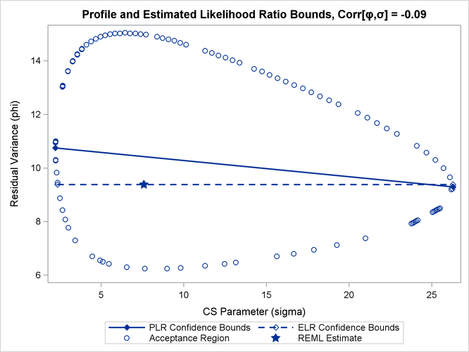
The major axes of the ellipse in Figure 41.11 are nearly aligned with the major axes of the coordinate system. As a consequence, the line connecting the PLR bounds passes
close to the REML estimate in the full model. As a result, ELR bounds will be similar to PLR bounds. Figure 41.12 displays a different scenario, a two-parameter AR(1) covariance structure with a more substantial correlation between the
AR(1) parameter (![]() ) and the residual variance (
) and the residual variance (![]() ).
).
Figure 41.12: PLR and ELR Intervals, Large Correlation between Parameters
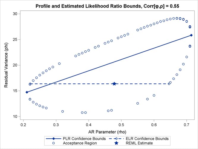
The correlation between the parameters yields an acceptance region whose major axes are not aligned with the axes of the coordinate
system. The ELR bound for ![]() passes through the REML estimate of
passes through the REML estimate of ![]() from the full model and is much shorter than the PLR interval. The PLR interval aligns with the major axis of the acceptance
region; it is the preferred confidence interval.
from the full model and is much shorter than the PLR interval. The PLR interval aligns with the major axis of the acceptance
region; it is the preferred confidence interval.