The GLIMMIX Procedure
-
Overview

-
Getting Started
-
SyntaxPROC GLIMMIX StatementBY StatementCLASS StatementCODE StatementCONTRAST StatementCOVTEST StatementEFFECT StatementESTIMATE StatementFREQ StatementID StatementLSMEANS StatementLSMESTIMATE StatementMODEL StatementNLOPTIONS StatementOUTPUT StatementPARMS StatementRANDOM StatementSLICE StatementSTORE StatementWEIGHT StatementProgramming StatementsUser-Defined Link or Variance Function
-
DetailsGeneralized Linear Models TheoryGeneralized Linear Mixed Models TheoryGLM Mode or GLMM ModeStatistical Inference for Covariance ParametersDegrees of Freedom MethodsEmpirical Covariance ("Sandwich") EstimatorsExploring and Comparing Covariance MatricesProcessing by SubjectsRadial Smoothing Based on Mixed ModelsOdds and Odds Ratio EstimationParameterization of Generalized Linear Mixed ModelsResponse-Level Ordering and ReferencingComparing the GLIMMIX and MIXED ProceduresSingly or Doubly Iterative FittingDefault Estimation TechniquesDefault OutputNotes on Output StatisticsODS Table NamesODS Graphics
-
ExamplesBinomial Counts in Randomized BlocksMating Experiment with Crossed Random EffectsSmoothing Disease Rates; Standardized Mortality RatiosQuasi-likelihood Estimation for Proportions with Unknown DistributionJoint Modeling of Binary and Count DataRadial Smoothing of Repeated Measures DataIsotonic Contrasts for Ordered AlternativesAdjusted Covariance Matrices of Fixed EffectsTesting Equality of Covariance and Correlation MatricesMultiple Trends Correspond to Multiple Extrema in Profile LikelihoodsMaximum Likelihood in Proportional Odds Model with Random EffectsFitting a Marginal (GEE-Type) ModelResponse Surface Comparisons with Multiplicity AdjustmentsGeneralized Poisson Mixed Model for Overdispersed Count DataComparing Multiple B-SplinesDiallel Experiment with Multimember Random EffectsLinear Inference Based on Summary DataWeighted Multilevel Model for Survey Data
- References
Recall from the section Notation for the Generalized Linear Mixed Model that
where ![]() and
and ![]() . Following Wolfinger and O’Connell (1993), a first-order Taylor series of
. Following Wolfinger and O’Connell (1993), a first-order Taylor series of ![]() about
about ![]() and
and ![]() yields
yields
where
is a diagonal matrix of derivatives of the conditional mean evaluated at the expansion locus. Rearranging terms yields the expression
The left side is the expected value, conditional on ![]() , of
, of
and
You can thus consider the model
which is a linear mixed model with pseudo-response ![]() , fixed effects
, fixed effects ![]() , random effects
, random effects ![]() , and
, and ![]() .
.
Now define
as the marginal variance in the linear mixed pseudo-model, where ![]() is the
is the ![]() parameter vector containing all unknowns in
parameter vector containing all unknowns in ![]() and
and ![]() . Based on this linearized model, an objective function can be defined, assuming that the distribution of
. Based on this linearized model, an objective function can be defined, assuming that the distribution of ![]() is known. The GLIMMIX procedure assumes that
is known. The GLIMMIX procedure assumes that ![]() has a normal distribution. The maximum log pseudo-likelihood (MxPL) and restricted log pseudo-likelihood (RxPL) for
has a normal distribution. The maximum log pseudo-likelihood (MxPL) and restricted log pseudo-likelihood (RxPL) for ![]() are then
are then
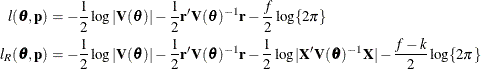
with ![]() . f denotes the sum of the frequencies used in the analysis, and k denotes the rank of
. f denotes the sum of the frequencies used in the analysis, and k denotes the rank of ![]() . The fixed-effects parameters
. The fixed-effects parameters ![]() are profiled from these expressions. The parameters in
are profiled from these expressions. The parameters in ![]() are estimated by the optimization techniques specified in the NLOPTIONS
statement. The objective function for minimization is
are estimated by the optimization techniques specified in the NLOPTIONS
statement. The objective function for minimization is ![]() or
or ![]() . At convergence, the profiled parameters are estimated and the random effects are predicted as
. At convergence, the profiled parameters are estimated and the random effects are predicted as
With these statistics, the pseudo-response and error weights of the linearized model are recomputed and the objective function
is minimized again. The predictors ![]() are the estimated BLUPs in the approximated linear model. This process continues until the relative change between parameter
estimates at two successive (outer) iterations is sufficiently small. See the PCONV=
option in the PROC GLIMMIX
statement for the computational details about how the GLIMMIX procedure compares parameter estimates across optimizations.
are the estimated BLUPs in the approximated linear model. This process continues until the relative change between parameter
estimates at two successive (outer) iterations is sufficiently small. See the PCONV=
option in the PROC GLIMMIX
statement for the computational details about how the GLIMMIX procedure compares parameter estimates across optimizations.
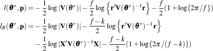
If the conditional distribution contains a scale parameter ![]() (Table 44.20), the GLIMMIX procedure profiles this parameter in GLMMs from the log pseudo-likelihoods as well. To this end define
(Table 44.20), the GLIMMIX procedure profiles this parameter in GLMMs from the log pseudo-likelihoods as well. To this end define
where ![]() is the covariance parameter vector with q – 1 elements. The matrices
is the covariance parameter vector with q – 1 elements. The matrices ![]() and
and ![]() are appropriately reparameterized versions of
are appropriately reparameterized versions of ![]() and
and ![]() . For example, if
. For example, if ![]() has a variance component structure and
has a variance component structure and ![]() , then
, then ![]() contains ratios of the variance components and
contains ratios of the variance components and ![]() , and
, and ![]() . The solution for
. The solution for ![]() is
is
where m = f for MxPL and m = f – k for RxPL. Substitution into the previous functions yields the profiled log pseudo-likelihoods,
Profiling of ![]() can be suppressed with the NOPROFILE
option in the PROC GLIMMIX
statement.
can be suppressed with the NOPROFILE
option in the PROC GLIMMIX
statement.
Where possible, the objective function, its gradient, and its Hessian employ the sweep-based W-transformation ( Hemmerle and Hartley 1973; Goodnight 1979; Goodnight and Hemmerle 1979). Further details about the minimization process in the general linear mixed model can be found in Wolfinger, Tobias, and Sall (1994).
The GLIMMIX procedure produces estimates of the variability of ![]() ,
, ![]() , and estimates of the prediction variability for
, and estimates of the prediction variability for ![]() ,
, ![]() . Denote as
. Denote as ![]() the matrix
the matrix
where all components on the right side are evaluated at the converged estimates. The mixed model equations (Henderson, 1984) in the linear mixed (pseudo-)model are then
and
![\begin{align*} \mb{C} & = \left[ \begin{array}{cc} \mb{X}’\mb{S}^{-1}\mb{X} & \mb{X}’\mb{S}^{-1}\mb{Z} \\ \mb{Z}’\mb{S}^{-1}\mb{X} & \mb{Z}’\mb{S}^{-1}\mb{Z} + \mb{G}(\widehat{\btheta })^{-1} \end{array} \right]^{-} \\ & = \left[ \begin{array}{cc} \widehat{\bOmega } & -\widehat{\bOmega }\mb{X}’\mb{V}(\widehat{\btheta })^{-1}\mb{Z}\mb{G}(\widehat{\btheta }) \\ -\mb{G}(\widehat{\btheta })\mb{Z}’\mb{V}(\widehat{\btheta })^{-1}\mb{X}\widehat{\bOmega } & \mb{M} + \mb{G}(\widehat{\btheta })\mb{Z}’\mb{V}(\widehat{\btheta })^{-1}\mb{X}\widehat{\bOmega } \mb{X}’\mb{V}(\widehat{\btheta })^{-1}\mb{ZG}(\widehat{\btheta }) \end{array} \right] \end{align*}](images/statug_glimmix0593.png)
is the approximate estimated variance-covariance matrix of ![]() . Here,
. Here, ![]() and
and ![]() .
.
The square roots of the diagonal elements of ![]() are reported in the Standard Error column of the "Parameter Estimates" table. This table is produced with the SOLUTION
option in the MODEL
statement. The prediction standard errors of the random-effects solutions are reported in the Std Err Pred column of the
"Solution for Random Effects" table. This table is produced with the SOLUTION
option in the RANDOM
statement.
are reported in the Standard Error column of the "Parameter Estimates" table. This table is produced with the SOLUTION
option in the MODEL
statement. The prediction standard errors of the random-effects solutions are reported in the Std Err Pred column of the
"Solution for Random Effects" table. This table is produced with the SOLUTION
option in the RANDOM
statement.
As a cautionary note, ![]() tends to underestimate the true sampling variability of [
tends to underestimate the true sampling variability of [![]() , because no account is made for the uncertainty in estimating
, because no account is made for the uncertainty in estimating ![]() and
and ![]() . Although inflation factors have been proposed (Kackar and Harville, 1984; Kass and Steffey, 1989; Prasad and Rao, 1990), they tend to be small for data sets that are fairly well balanced. PROC GLIMMIX does not compute any inflation factors
by default. The DDFM=
KENWARDROGER option in the MODEL
statement prompts PROC GLIMMIX to compute a specific inflation factor (Kenward and Roger, 1997), along with Satterthwaite-based degrees of freedom.
. Although inflation factors have been proposed (Kackar and Harville, 1984; Kass and Steffey, 1989; Prasad and Rao, 1990), they tend to be small for data sets that are fairly well balanced. PROC GLIMMIX does not compute any inflation factors
by default. The DDFM=
KENWARDROGER option in the MODEL
statement prompts PROC GLIMMIX to compute a specific inflation factor (Kenward and Roger, 1997), along with Satterthwaite-based degrees of freedom.
If ![]() is singular, or if you use the CHOL
option of the PROC GLIMMIX
statement, the mixed model equations are modified as follows. Let
is singular, or if you use the CHOL
option of the PROC GLIMMIX
statement, the mixed model equations are modified as follows. Let ![]() denote the lower triangular matrix so that
denote the lower triangular matrix so that ![]() . PROC GLIMMIX then solves the equations
. PROC GLIMMIX then solves the equations
and transforms ![]() and a generalized inverse of the left-side coefficient matrix by using
and a generalized inverse of the left-side coefficient matrix by using ![]() .
.
The asymptotic covariance matrix of the covariance parameter estimator ![]() is computed based on the observed or expected Hessian matrix of the optimization procedure. Consider first the case where
the scale parameter
is computed based on the observed or expected Hessian matrix of the optimization procedure. Consider first the case where
the scale parameter ![]() is not present or not profiled. Because
is not present or not profiled. Because ![]() is profiled from the pseudo-likelihood, the objective function for minimization is
is profiled from the pseudo-likelihood, the objective function for minimization is ![]() for METHOD=
MSPL and METHOD=
MMPL and
for METHOD=
MSPL and METHOD=
MMPL and ![]() for METHOD=
RSPL and METHOD=
RMPL. Denote the observed Hessian (second derivative) matrix as
for METHOD=
RSPL and METHOD=
RMPL. Denote the observed Hessian (second derivative) matrix as
The GLIMMIX procedure computes the variance of ![]() by default as
by default as ![]() . If the Hessian is not positive definite, a sweep-based generalized inverse is used instead. When the EXPHESSIAN
option of the PROC GLIMMIX
statement is used, or when the procedure is in scoring mode at convergence (see the SCORING
option in the PROC GLIMMIX
statement), the observed Hessian is replaced with an approximated expected Hessian matrix in these calculations.
. If the Hessian is not positive definite, a sweep-based generalized inverse is used instead. When the EXPHESSIAN
option of the PROC GLIMMIX
statement is used, or when the procedure is in scoring mode at convergence (see the SCORING
option in the PROC GLIMMIX
statement), the observed Hessian is replaced with an approximated expected Hessian matrix in these calculations.
Following Wolfinger, Tobias, and Sall (1994), define the following components of the gradient and Hessian in the optimization:
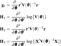
Table 44.23 gives expressions for the Hessian matrix ![]() depending on estimation method, profiling, and scoring.
depending on estimation method, profiling, and scoring.
Table 44.23: Hessian Computation in GLIMMIX
|
Profiling |
Scoring |
MxPL |
RxPL |
|---|---|---|---|
|
No |
No |
|
|
|
No |
Yes |
|
|
|
No |
Modified |
|
|
|
Yes |
No |
|
|
|
Yes |
Yes |
|
|
|
Yes |
Modified |
|
|
The "Modified" expressions for the Hessian under scoring in RxPL estimation refer to a modified scoring method. In some cases, the modification leads to faster convergence than the standard scoring algorithm. The modification is requested with the SCOREMOD option in the PROC GLIMMIX statement.
Finally, in the case of a profiled scale parameter ![]() , the Hessian for the
, the Hessian for the ![]() parameterization is converted into that for the
parameterization is converted into that for the ![]() parameterization as
parameterization as
where
![\[ \mb{B} = \left[ \begin{array}{ccccc} 1/\phi & 0 & \cdots & 0 & 0 \\ 0 & 1/\phi & \cdots & 0 & 0 \\ 0 & \cdots & \cdots & 1/\phi & 0 \\ -\theta ^*_1/\phi & -\theta ^*_2/\phi & \cdots & -\theta _{q-1}^*/\phi & 1 \end{array}\right] \]](images/statug_glimmix0620.png)
There are two basic choices for the expansion locus of the linearization. A subject-specific (SS) expansion uses
which are the current estimates of the fixed effects and estimated BLUPs. The population-averaged (PA) expansion expands about the same fixed effects and the expected value of the random effects
To recompute the pseudo-response and weights in the SS expansion, the BLUPs must be computed every time the objective function
in the linear mixed model is maximized. The PA expansion does not require any BLUPs. The four pseudo-likelihood methods implemented
in the GLIMMIX procedure are the ![]() factorial combination between two expansion loci and residual versus maximum pseudo-likelihood estimation. The following
table shows the combination and the corresponding values of the METHOD=
option (PROC GLIMMIX
statement); METHOD=
RSPL is the default.
factorial combination between two expansion loci and residual versus maximum pseudo-likelihood estimation. The following
table shows the combination and the corresponding values of the METHOD=
option (PROC GLIMMIX
statement); METHOD=
RSPL is the default.
|
Type of |
Expansion Locus |
|
|---|---|---|
|
PL |
|
E |
|
residual |
RSPL |
RMPL |
|
maximum |
MSPL |
MMPL |