The PHREG Procedure
- Overview
-
Getting Started

-
Syntax
 PROC PHREG StatementASSESS StatementBASELINE StatementBAYES StatementBY StatementCLASS StatementCONTRAST StatementEFFECT StatementESTIMATE StatementFREQ StatementHAZARDRATIO StatementID StatementLSMEANS StatementLSMESTIMATE StatementMODEL StatementOUTPUT StatementProgramming StatementsRANDOM StatementSTRATA StatementSLICE StatementSTORE StatementTEST StatementWEIGHT Statement
 -
Details
 Failure Time DistributionTime and CLASS Variables UsagePartial Likelihood Function for the Cox ModelCounting Process Style of InputLeft-Truncation of Failure TimesThe Multiplicative Hazards ModelThe Frailty ModelHazard RatiosProportional Rates/Means Models for Recurrent EventsNewton-Raphson MethodFirth’s Modification for Maximum Likelihood EstimationRobust Sandwich Variance EstimateTesting the Global Null HypothesisType 3 TestsConfidence Limits for a Hazard RatioUsing the TEST Statement to Test Linear HypothesesAnalysis of Multivariate Failure Time DataModel Fit StatisticsResidualsDiagnostics Based on Weighted ResidualsInfluence of Observations on Overall Fit of the ModelSurvivor Function EstimatorsEffect Selection MethodsAssessment of the Proportional Hazards ModelThe Penalized Partial Likelihood Approach for Fitting Frailty ModelsSpecifics for Bayesian AnalysisComputational ResourcesInput and Output Data SetsDisplayed OutputODS Table NamesODS Graphics
 -
Examples
 Stepwise RegressionBest Subset SelectionModeling with Categorical PredictorsFirth’s Correction for Monotone LikelihoodConditional Logistic Regression for m:n MatchingModel Using Time-Dependent Explanatory VariablesTime-Dependent Repeated Measurements of a CovariateSurvival CurvesAnalysis of ResidualsAnalysis of Recurrent Events DataAnalysis of Clustered DataModel Assessment Using Cumulative Sums of Martingale ResidualsBayesian Analysis of the Cox ModelBayesian Analysis of Piecewise Exponential Model
 - References
Example 67.8 Survival Curves
You might want to use your regression analysis results to predict the survivorship of subjects of specific covariate values.
The COVARIATES= data set in the BASELINE statement enables you to specify the sets of covariate values for the prediction.
On the other hand, you might want to summarize the survival experience of an average patient for a given population. The DIRADJ
option in the BASELINE statement computes the direct adjusted survival curve that averages the estimated survival curves for
patients whose covariates are represented in the COVARIATES= data set. By using the PLOTS= option in the PROC PHREG statement,
you can use ODS Graphics to display the predicted survival curves. You can elect to output the predicted survival curves in
a SAS data set by optionally specifying the OUT= option in the BASELINE statement. This example illustrates how to obtain
the covariate-specific survival curves and the direct adjusted survival curve by using the Myeloma data set in Example 67.1, where variables LogBUN and HGB were identified as the most important prognostic factors.
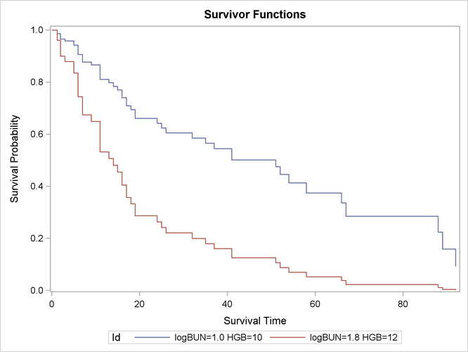
Suppose you want to compute the predicted survival curves for two sets of covariate values: (LogBUN=1.0, HGB=10) and (LogBUN=1.8, HGB=12). These values are saved in the data set Inrisks in the following DATA step. Also created in this data set is the variable Id, whose values will be used in identifying the covariate sets in the survival plot.
data Inrisks;
   length Id $20;
   input LogBUN HGB Id $12-31;
   datalines;
1.00 10.0  logBUN=1.0 HGB=10
1.80 12.0  logBUN=1.8 HGB=12
;
The following statements plot the survival functions in Output 67.8.1 and save the survival estimates in the data set Pred1:
ods graphics on;
proc phreg data=Myeloma plots(overlay)=survival;
   model Time*VStatus(0)=LogBUN HGB;
   baseline covariates=Inrisks out=Pred1 survival=_all_/rowid=Id;
run;
The COVARIATES= option in the BASELINE statement specifies the data set that contains the set of covariates of interest. The
PLOTS= option in the PROC PHREG statement creates the survival plot. The OVERLAY suboption overlays the two curves in the
same plot. If the OVERLAY suboption is not specified, each curve is displayed in a separate plot. The ROWID= option in the
BASELINE statement specifies that the values of the variable Id in the COVARIATES= data set be used to identify the curves in the plot. The SURVIVAL=_ALL_ option in the BASELINE statement
requests that the estimated survivor function, standard error, and lower and upper confidence limits for the survivor function
be output into the SAS data set that is specified in the OUT= option.
The survival Plot (Output 67.8.1) contains two curves, one for each of row of covariates in the data set Inrisks.
Output 67.8.1: Estimated Survivor Function Plot

The following statements print out the observations in the data set Pred1 for the realization LogBUN=1.00 and HGB=10.0:
proc print data=Pred1(where=(logBUN=1 and HGB=10));
run;
As shown in Output 67.8.2, 32 observations represent the survivor function for the realization LogBUN=1.00 and HGB=10.0. The first observation has survival time 0 and survivor function estimate 1.0. Each of the remaining 31 observations
represents a distinct event time in the input data set Myeloma. These observations are presented in ascending order of the event times. Note that all the variables in the COVARIATES=InRisks data set are included in the OUT=Pred1 data set. Likewise, you can print out the observations that represent the survivor function for the realization LogBUN=1.80 and HGB=12.0.
Output 67.8.2: Survivor Function Estimates for LogBUN=1.0 and HGB=10.0
| Obs | Id | LogBUN | HGB | Time | Survival | StdErrSurvival | LowerSurvival | UpperSurvival |
|---|---|---|---|---|---|---|---|---|
| 1 | logBUN=1.0 HGB=10 | 1 | 10 | 0.00 | 1.00000 | . | . | . |
| 2 | logBUN=1.0 HGB=10 | 1 | 10 | 1.25 | 0.98678 | 0.01043 | 0.96655 | 1.00000 |
| 3 | logBUN=1.0 HGB=10 | 1 | 10 | 2.00 | 0.96559 | 0.01907 | 0.92892 | 1.00000 |
| 4 | logBUN=1.0 HGB=10 | 1 | 10 | 3.00 | 0.95818 | 0.02180 | 0.91638 | 1.00000 |
| 5 | logBUN=1.0 HGB=10 | 1 | 10 | 5.00 | 0.94188 | 0.02747 | 0.88955 | 0.99729 |
| 6 | logBUN=1.0 HGB=10 | 1 | 10 | 6.00 | 0.90635 | 0.03796 | 0.83492 | 0.98389 |
| 7 | logBUN=1.0 HGB=10 | 1 | 10 | 7.00 | 0.87742 | 0.04535 | 0.79290 | 0.97096 |
| 8 | logBUN=1.0 HGB=10 | 1 | 10 | 9.00 | 0.86646 | 0.04801 | 0.77729 | 0.96585 |
| 9 | logBUN=1.0 HGB=10 | 1 | 10 | 11.00 | 0.81084 | 0.05976 | 0.70178 | 0.93686 |
| 10 | logBUN=1.0 HGB=10 | 1 | 10 | 13.00 | 0.79800 | 0.06238 | 0.68464 | 0.93012 |
| 11 | logBUN=1.0 HGB=10 | 1 | 10 | 14.00 | 0.78384 | 0.06515 | 0.66601 | 0.92251 |
| 12 | logBUN=1.0 HGB=10 | 1 | 10 | 15.00 | 0.76965 | 0.06779 | 0.64762 | 0.91467 |
| 13 | logBUN=1.0 HGB=10 | 1 | 10 | 16.00 | 0.74071 | 0.07269 | 0.61110 | 0.89781 |
| 14 | logBUN=1.0 HGB=10 | 1 | 10 | 17.00 | 0.71005 | 0.07760 | 0.57315 | 0.87966 |
| 15 | logBUN=1.0 HGB=10 | 1 | 10 | 18.00 | 0.69392 | 0.07998 | 0.55360 | 0.86980 |
| 16 | logBUN=1.0 HGB=10 | 1 | 10 | 19.00 | 0.66062 | 0.08442 | 0.51425 | 0.84865 |
| 17 | logBUN=1.0 HGB=10 | 1 | 10 | 24.00 | 0.64210 | 0.08691 | 0.49248 | 0.83717 |
| 18 | logBUN=1.0 HGB=10 | 1 | 10 | 25.00 | 0.62360 | 0.08921 | 0.47112 | 0.82542 |
| 19 | logBUN=1.0 HGB=10 | 1 | 10 | 26.00 | 0.60523 | 0.09136 | 0.45023 | 0.81359 |
| 20 | logBUN=1.0 HGB=10 | 1 | 10 | 32.00 | 0.58549 | 0.09371 | 0.42784 | 0.80122 |
| 21 | logBUN=1.0 HGB=10 | 1 | 10 | 35.00 | 0.56534 | 0.09593 | 0.40539 | 0.78840 |
| 22 | logBUN=1.0 HGB=10 | 1 | 10 | 37.00 | 0.54465 | 0.09816 | 0.38257 | 0.77542 |
| 23 | logBUN=1.0 HGB=10 | 1 | 10 | 41.00 | 0.50178 | 0.10166 | 0.33733 | 0.74639 |
| 24 | logBUN=1.0 HGB=10 | 1 | 10 | 51.00 | 0.47546 | 0.10368 | 0.31009 | 0.72901 |
| 25 | logBUN=1.0 HGB=10 | 1 | 10 | 52.00 | 0.44510 | 0.10522 | 0.28006 | 0.70741 |
| 26 | logBUN=1.0 HGB=10 | 1 | 10 | 54.00 | 0.41266 | 0.10689 | 0.24837 | 0.68560 |
| 27 | logBUN=1.0 HGB=10 | 1 | 10 | 58.00 | 0.37465 | 0.10891 | 0.21192 | 0.66232 |
| 28 | logBUN=1.0 HGB=10 | 1 | 10 | 66.00 | 0.33626 | 0.10980 | 0.17731 | 0.63772 |
| 29 | logBUN=1.0 HGB=10 | 1 | 10 | 67.00 | 0.28529 | 0.11029 | 0.13372 | 0.60864 |
| 30 | logBUN=1.0 HGB=10 | 1 | 10 | 88.00 | 0.22412 | 0.10928 | 0.08619 | 0.58282 |
| 31 | logBUN=1.0 HGB=10 | 1 | 10 | 89.00 | 0.15864 | 0.10317 | 0.04435 | 0.56750 |
| 32 | logBUN=1.0 HGB=10 | 1 | 10 | 92.00 | 0.09180 | 0.08545 | 0.01481 | 0.56907 |
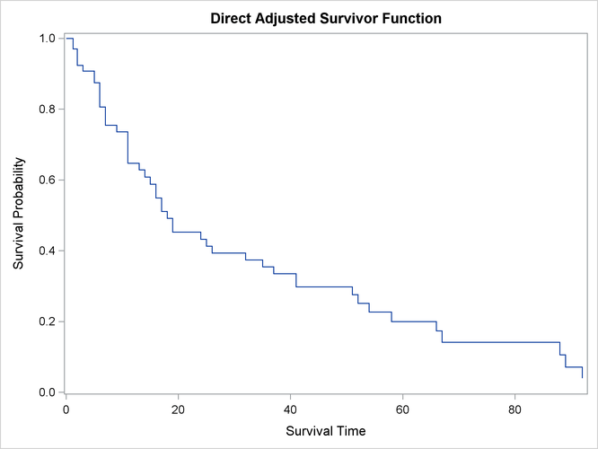
Next, the DIRADJ option in the BASELINE statement is used to request a survival curve that represents the survival experience of an average patient in the population in which the COVARIATES= data set is sampled. When the DIRADJ option is specified, PROC PHREG computes the direct adjusted survival function by averaging the predicted survival functions for the rows in the COVARIATES= data set. The following statements plot the direct adjusted survival function in Output 67.8.3.
proc phreg data=Myeloma plots=survival;
   model Time*VStatus(0)=LogBUN HGB;
   baseline covariates=Myeloma survival=_all_/diradj;
run;
When the DIRADJ option is specified in the BASELINE statement, the default COVARIATES= data set is the input data set. For clarity, the COVARIATES=MYELOMA is specified in the BASELINE statement in the preceding PROC PHREG call.
Output 67.8.3: Average Survival Function for the Myeloma Data

If neither the COVARIATES= data set nor the DIRADJ option is specified in the BASELINE statement, PROC PHREG computes a predicted
survival curve based on ![]() , the average values of the covariate vectors in the input data (Neuberger et al., 1986). This curve represents the survival experience of a patient with an average prognostic index
, the average values of the covariate vectors in the input data (Neuberger et al., 1986). This curve represents the survival experience of a patient with an average prognostic index ![]() equal to the average prognostic index of all patients. This approach has a couple of drawbacks: it is possible that no patient
could ever have such an average index, and it does not account for the variability in the prognostic factor from patient to
patient.
equal to the average prognostic index of all patients. This approach has a couple of drawbacks: it is possible that no patient
could ever have such an average index, and it does not account for the variability in the prognostic factor from patient to
patient.
The DIRADJ option is particularly useful if the model contains a categorical explanatory variable that represents different
treatments of interest. By specifying this categorical variable in the GROUP= option, you obtain a direct adjusted survival
curve for each category of the variable. In addition, you can use the OUTDIFF= option to save all pairwise differences of
these direct adjusted survival probabilities in a data set. For illustration, consider a model that also includes the categorical
variable Frac, which has a value 0 if a patient did not have a fracture at diagnosis and 1 otherwise, as an explanatory variable. The following
statements plot the adjusted survival curves in Output 67.8.4 and save the differences of the direct adjusted survival probabilities in the data set Diff1:
proc phreg data=Myeloma plots(overlay)=survival;
   class Frac;
   model Time*VStatus(0)=LogBUN HGB Frac;
   baseline covariates=Myeloma outdiff=Diff1 survival=_all_/diradj group=Frac;
run;
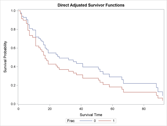
Because the CLASS variable Frac is specified as the GROUP= variable, a separate direct adjusted survival curve is computed for each value of the variable
Frac. Each direct adjusted survival curve is the average of the predicted survival curves for all the patients in the entire Myeloma data set with their Frac value set to a specific constant. For example, the direct adjusted survival curve for Frac=0 (no fracture at diagnosis) is computed as follows:
-
The value of the variable
Fracis set to 0 for all observations in theMyelomadata set. -
The survival curve for each observation in the modified data set is computed.
-
All the survival curves computed in step 2 are averaged.
Output 67.8.4: Average Survival by Fracture Status

Output 67.8.4 shows that patients without fracture at diagnosis have better survival than those with fractures. Differences in the survival probabilities and their standard errors are displayed in Output 67.8.5.
proc print data=Diff1;
run;
ods graphics off;
Output 67.8.5: Differences in the Survival between Fracture and Nonfracture
| Obs | Frac | Frac2 | Time | SurvDiff | StdErr |
|---|---|---|---|---|---|
| 1 | 0 | 1 | 1.25 | 0.01074 | 0.01199 |
| 2 | 0 | 1 | 2.00 | 0.02653 | 0.02605 |
| 3 | 0 | 1 | 3.00 | 0.03165 | 0.03063 |
| 4 | 0 | 1 | 5.00 | 0.04191 | 0.03963 |
| 5 | 0 | 1 | 6.00 | 0.06115 | 0.05669 |
| 6 | 0 | 1 | 7.00 | 0.07416 | 0.06853 |
| 7 | 0 | 1 | 9.00 | 0.07854 | 0.07261 |
| 8 | 0 | 1 | 11.00 | 0.09669 | 0.09002 |
| 9 | 0 | 1 | 13.00 | 0.09998 | 0.09327 |
| 10 | 0 | 1 | 14.00 | 0.10319 | 0.09644 |
| 11 | 0 | 1 | 15.00 | 0.10611 | 0.09937 |
| 12 | 0 | 1 | 16.00 | 0.11117 | 0.10464 |
| 13 | 0 | 1 | 17.00 | 0.11532 | 0.10922 |
| 14 | 0 | 1 | 18.00 | 0.11704 | 0.11120 |
| 15 | 0 | 1 | 19.00 | 0.11969 | 0.11447 |
| 16 | 0 | 1 | 24.00 | 0.12072 | 0.11593 |
| 17 | 0 | 1 | 25.00 | 0.12145 | 0.11713 |
| 18 | 0 | 1 | 26.00 | 0.12189 | 0.11808 |
| 19 | 0 | 1 | 32.00 | 0.12208 | 0.11883 |
| 20 | 0 | 1 | 35.00 | 0.12197 | 0.11933 |
| 21 | 0 | 1 | 37.00 | 0.12155 | 0.11956 |
| 22 | 0 | 1 | 41.00 | 0.11983 | 0.11924 |
| 23 | 0 | 1 | 51.00 | 0.11821 | 0.11850 |
| 24 | 0 | 1 | 52.00 | 0.11580 | 0.11714 |
| 25 | 0 | 1 | 54.00 | 0.11262 | 0.11507 |
| 26 | 0 | 1 | 58.00 | 0.10824 | 0.11203 |
| 27 | 0 | 1 | 66.00 | 0.10301 | 0.10814 |
| 28 | 0 | 1 | 67.00 | 0.09451 | 0.10130 |
| 29 | 0 | 1 | 88.00 | 0.08248 | 0.09133 |
| 30 | 0 | 1 | 89.00 | 0.06847 | 0.08033 |
| 31 | 0 | 1 | 92.00 | 0.05038 | 0.06515 |